Stochastic Gradient Descent (SGD)

Author: Seyed Rasoul Mortazavi

Stochastic Gradient Descent (SGD) is a widely used optimization algorithm in machine learning and deep learning. It’s a variant of gradient descent that’s particularly useful when dealing with large datasets.

What is Gradient Descent?

Before understanding SGD, it’s crucial to grasp the concept of gradient descent. In optimization, we often aim to minimize a cost function (also known as objective function). This function represents the error of a model’s predictions. Gradient descent is an iterative algorithm that finds the minimum of this function by repeatedly taking steps in the direction of the steepest descent (the negative gradient).

How Gradient Descent Works:

Initialization: Start with an initial guess(usually random) for the model’s parameters (e.g., weights in a neural network).
Gradient Calculation: Compute the gradient of the cost function with respect to the parameters. The gradient points in the direction of the steepest ascent.
Parameter Update: Move the parameters in the opposite direction of the gradient to descend towards the minimum. The step size is controlled by the learning rate (a hyperparameter).
Iteration: Repeat steps 2 and 3 until the algorithm converges to a minimum (or a satisfactory level of accuracy).

What is Stochastic Gradient Descent?

SGD differs from standard (batch) gradient descent in how it calculates the gradient:

Batch Gradient Descent: Computes the gradient using all training examples in each iteration. This is computationally expensive for large datasets.
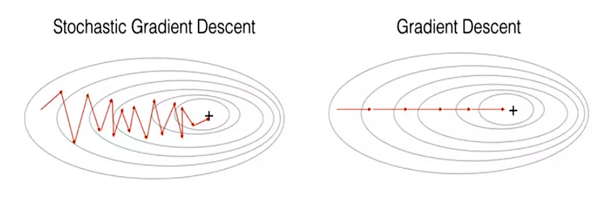
Stochastic Gradient Descent: Computes the gradient using only one randomly chosen training example in each iteration. This significantly speeds up each iteration.

Key Characteristics of SGD:

Stochasticity (Randomness): Using a single random data point introduces randomness into the optimization process. This causes the algorithm to “zig-zag” towards the minimum, rather than taking a direct path.

SGD vs GD

Faster Iterations: Each iteration is computationally much cheaper than in batch gradient descent, making SGD suitable for large datasets.
Noise and Fluctuations: The noisy updates can help the algorithm escape local minima and potentially find a better global minimum.
Learning Rate Sensitivity: SGD is sensitive to the choice of the learning rate. A large learning rate can cause divergence, while a small learning rate can lead to slow convergence.

Simplified Algorithm:

$ \text{Initialize parameters w}$

$ \text{For each iteration (iteration over the entire dataset):}$

$ \text{Shuffle the training data}$

$ \text{For each training example (xᵢ, yᵢ):}$

$ \text{Calculate the gradient of the cost function with respect to w using (xᵢ, yᵢ)}$

$ \text{Update w: w = w - learning_rate * gradient }$

Advantages of SGD:

Computational Efficiency: Especially for large datasets.
Escape from Local Minima: The inherent noise can help the algorithm escape shallow local minima.

Disadvantages of SGD:

Noisy Updates: The zig-zagging can make precise convergence difficult.
Learning Rate Tuning: Finding a suitable learning rate can be challenging.

Weight update formula:

The weight update rule in SGD is:

\[w_{t+1} = w_t - \eta \nabla_w J(w_t)\]

Where:

($w_{t+1}$): Weight at iteration t+1
($w_t$): Weight at iteration t
($\eta$): Learning rate
($\nabla J(w_t)$): Gradient of the cost function J with respect to w at iteration t using training example (xᵢ, yᵢ)
Weight Update Formula using Taylor Expansion

Taylor Expansion of $J(w + \Delta w)$

Assume $J(w)$ is quadratic in $w$, e.g. $J(w)=aw^2+bw+c$ with $a\neq0$.

\[J(w + \Delta w) = J(w) + \frac{\Delta w}{1!} J'(w) + \frac{(\Delta w)^2}{2!} J''(w) + \dots\]

Simplifying the Expansion

Let the second–order term be:

\[b = \frac{1}{2} J''(w)\]

Then:

\[J(w + \Delta w) = J(w) + \Delta w \, J'(w) + (\Delta w)^2 b\]

\[J(w + \Delta w) - J(w) = \Delta w \, \nabla_w J(w) + (\Delta w)^2 b\]

Define

\[J_1(\Delta w) = J(w + \Delta w) - J(w)\]

Thus

\[J_1(\Delta w) = \Delta w \, \nabla_w J(w) + (\Delta w)^2 b\]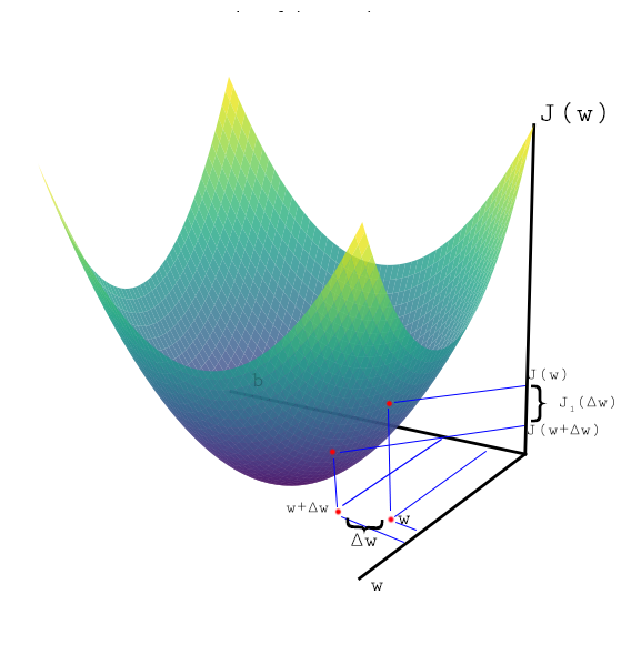

delta w

Taking the Derivative of $J_1(\Delta w)$ with respect to $\Delta w$

To reach the optimal (minimum) point of J(w) as quickly as possible, we need to find the optimal Δw. Therefore, we take the derivative of j₁(w) with respect to Δw and set it to zero to find the best Δw. $\frac{\partial J_1(\Delta w)}{\partial \Delta w} = \nabla_w J(w) + 2b\Delta w = 0$

Solving for $ \Delta w $

\[\Delta w = - \frac{1}{2b}\nabla_w J(w)\]

Rewriting

$\Delta w = w_{\text{new}} - w_{\text{old}}$

$\frac{1}{2b} = \eta$ $w_{\text{new}} - w_{\text{old}} = - \eta \cdot \nabla_w J(w)$

Thus, the update rule becomes:

$w_{\text{new}} = w_{\text{old}} - \eta \cdot \nabla_w J(w)$

$\eta$ also known as Learning Rate or Step Size

If l(e) is square error so: $J(w) = E\{error^2\}$ $error = y - \hat y = y-w^T.x+b$ $\nabla_w J(w)= 2\cdot error \cdot \frac{\partial error}{\partial w}$ $\nabla_w J(w)= 2\cdot error \cdot (-x)$ $w_{\text{new}} =w_{\text{old}} - \eta \cdot 2\cdot error \cdot (-x)$

SGD In Practice

import numpy as np
import matplotlib.pyplot as plt

# Initial settings
real_w = np.array([5, 3, 8])  # Actual weights including bias: [w1, w2, b]
learning_rate = 0.005  # Learning rate
w = np.random.randn(len(real_w))  # Random initialization of weights
epsilon = 1e-5  # Stopping condition
max_iterations = 10000  # Maximum number of iterations

# Histories for visualization
error_history = []
w_history = [w.copy()]

# Data generation function
def generate_data(with_noise=True):
    x = np.random.uniform(0, 10, size=(len(real_w) - 1, 1))  # Generate input data
    x = np.append(x, [1])  # Add bias to the input data
    y = np.dot(real_w, x)  # Compute the actual output
    if with_noise:
        y += np.random.normal(0, 0.5)  # Add noise to the output
    return x, y

# Initializing the cost function
J_old = float('inf')
J_new = 0

print(f"real w:", real_w)

# Training loop for SGD
for iteration in range(max_iterations):
    x, y = generate_data(with_noise=True)
    
    y_hat = np.dot(w, x)  # Compute the predicted output
    error = y - y_hat  # Compute the error
    J_new = error**2  # Compute the cost function (squared error)
    
    # Update weights
    w = w - learning_rate * (2 * error * -x)  # Update rule: w - eta * gradient(J)
    
    # Save history
    error_history.append(J_new)
    w_history.append(w.copy())
    
    # Display weights at each iteration
    print(f"Iteration {iteration + 1}: Weights = {w}")
    
    # Stopping condition
    if abs(J_new - J_old) < epsilon:
        print(f"Stopping at iteration {iteration + 1}, change in cost: {abs(J_new - J_old)}")
        break
    
    J_old = J_new

# Display final results
print("\n\nInitial weights:", w_history[0])
print("Final weights:", w)
print("Real weights:", real_w)

# --- Training Visualizations ---

# Plot Error by Iterations
plt.figure(figsize=(8, 5))
plt.plot(error_history, color='red')
plt.title("Error by Iterations (SGD)")
plt.xlabel("Iteration")
plt.ylabel("Squared Error")
plt.grid(True)
plt.show()

# Plot Learning Curve (all weights)
w_history = np.array(w_history)
plt.figure(figsize=(8, 5))
label_list = [f'w{i}(real={real_w[i-1]})' for i in range(1, len(w) + 1)]
plt.plot(w_history, label=label_list)
plt.title("Learning Curve")
plt.xlabel("Iteration")
plt.ylabel("Weight Values")
plt.legend()
plt.grid(True)
plt.show()

Applications Of SGD:

Training Deep Neural Networks:: SGD and its variants, particularly Adam and RMSProp, are extensively used in training deep neural networks (DNNs). These optimization algorithms enable efficient training of DNNs with millions of parameters, facilitating breakthroughs in computer vision, natural language processing, and reinforcement learning.
Linear and Logistic Regression: SGD is a fundamental optimization technique for training linear and logistic regression models. Its ability to handle large datasets and converge quickly makes it well-suited for finance, healthcare, and marketing regression tasks.
Recommender Systems: SGD is instrumental in training collaborative filtering models for recommender systems. These models use SGD to learn user preferences and make personalized recommendations in e-commerce, streaming, and social media platforms.
Online Learning: SGD’s ability to adapt to streaming data and non-stationary environments makes it well-suited for online learning scenarios. Online learning applications include real-time anomaly detection, personalized content recommendation, and adaptive control systems.
Generative Adversarial Networks (GANs): SGD optimization algorithms train generative adversarial networks (GANs) for generating realistic images, videos, and audio. GANs trained with SGD are used in art generation, image editing, and data augmentation.

Conclusion:

SGD (Stochastic Gradient Descent) is a fast, scalable, and widely used optimization algorithm for machine learning, especially with large datasets. Instead of calculating the gradient over the entire dataset like batch gradient descent, SGD updates model parameters using the gradient computed from a single, randomly chosen data point (or a small mini-batch) in each iteration. This makes each update much faster but introduces noise, causing the optimization path to “zig-zag” towards the minimum. This noise, however, can help escape local minima. Key considerations are the learning rate (which controls the step size) and the use of variants like mini-batch SGD, momentum, and adaptive learning rate methods (e.g., Adam, RMSprop) to improve convergence speed and stability. In short, SGD prioritizes speed and scalability over precise convergence, making it a powerful tool for training complex models on large datasets.