LMS (Least Mean Squares) and RBF (Radial Basis Function)

Least Mean Squares (LMS) Algorithm

The LMS algorithm is an adaptive algorithm used to minimize the mean squared error (MSE) between the actual output of a system and the desired output. It is commonly applied in signal processing, adaptive filtering, and machine learning.

Steps of the LMS Algorithm

Given:

Input vector: $ \mathbf{x}(n) = [x_1(n), x_2(n), \ldots, x_d(n)]^T $
Desired output: $ d(n) $
Current weight vector: $ \mathbf{w}(n) = [w_1(n), w_2(n), \ldots, w_d(n)]^T $

Step 1: Compute the actual output

$y(n) = \mathbf{w}^T(n) \cdot \mathbf{x}(n)$

Step 2: Calculate the error

$e(n) = d(n) - y(n)$

Step 3: Update the weights

$\mathbf{w}(n+1) = \mathbf{w}(n) + \mu e(n) \mathbf{x}(n)$ Where:

$ \mu $ is the learning rate, which controls the step size of the weight updates. A small $ \mu $ ensures stability but slows down convergence, while a large $ \mu $ may lead to instability.

Key Features of LMS

Simplicity: Easy to implement.
Online learning: Can be updated iteratively with new data.
Convergence: Depends on the choice of $ \mu $. Proper tuning is required to balance speed and stability.

Applications of LMS

Adaptive noise cancellation.
Channel equalization in communication systems.
Echo cancellation in telephony.

Radial Basis Function (RBF) Networks

An RBF network is a type of artificial neural network that uses radial basis functions as its activation functions. It is well-suited for function approximation, classification, and interpolation tasks.

Structure of an RBF Network

Input Layer: Passes the input vector $ \mathbf{x} $ directly to the hidden layer.
Hidden Layer:
- Each neuron in the hidden layer computes a radial basis function of the input.
- Common radial basis function: Gaussian function
  $\phi(\mathbf{x}) = \exp\left(-\frac{\|\mathbf{x} - \mu\|^2}{2\sigma^2}\right)$ Where:
  - $ \mu $ is the center of the radial basis function.
  - $ \sigma $ is the spread or width of the Gaussian.
Output Layer:
- Computes a weighted sum of the hidden layer outputs to produce the final output.
  $y(\mathbf{x}) = \sum_{i=1}^{M} w_i \phi_i(\mathbf{x})$ Where $ M $ is the number of hidden neurons, and $ w_i $ are the output weights.

Learning Process in RBF Networks

Center selection:
The centers $ \mathbf{c}_i $ can be selected using:
- Clustering methods such as k-means.
- Random selection from the input data.
Width selection ($\sigma$):
The width of the Gaussian functions can be set based on:
- The distance between neighboring centers.
- A fixed value for all neurons.
Weight determination:
Once the centers and widths are fixed, the output layer weights $ w_i $ are computed using a least squares method to minimize the error between the network output and the desired output.

Combining LMS with RBF Networks

When using LMS with an RBF network, the LMS algorithm is employed to adaptively update the output weights of the RBF network to minimize the error between the predicted output and the desired output.

LMS RBF

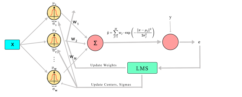
Steps in LMS-RBF

Compute the output of the RBF network using the current weights.
Calculate the error between the desired output and the network output.
Update the output weights, centers and sigmas using the LMS rule: $w_{j,k+1} = w_{j,k} - \eta \cdot \frac{\partial J}{\partial w_{j,k}}$
\[\mu_{j,k+1} = \mu_{j,k} - \eta \cdot \frac{\partial J}{\partial \mu_{j,k}}\] \[\sigma_{j,k+1} = \sigma_{j,k} - \eta \cdot \frac{\partial J}{\partial \sigma_{j,k}}\]

Advantages of LMS-RBF

Fast training: Since LMS updates are simple and efficient, the training process can be faster compared to gradient-based methods.
Adaptive learning: LMS allows the RBF network to adapt in real-time to changing inputs or environments.
Good for online learning: The combination works well for applications where data arrives sequentially, and the model needs to update continuously.

Applications of LMS-RBF

Real-time control systems.
Time series prediction.
Pattern recognition and classification.
Signal processing and adaptive filtering.
Update Rules

\[e_k = y - \sum_{i} w_j \cdot \exp\left(-\frac{\|x - \mu_j\|^2}{2 \sigma_j^2}\right)\] \[J = e_k^2=(y - \sum_{i} w_j \cdot \exp\left(-\frac{\|x - \mu_j\|^2}{2 \sigma_j^2}\right))^2\]

Update Rule For $w_j$:

$w_{j,k+1} = w_{j,k} - \eta \cdot \frac{\partial J}{\partial w_{j,k}}$

\[\frac{\partial J}{\partial w_{j,k}} = 2e_k \cdot \frac{\partial e_k}{\partial w_{j,k}}\] \[\frac{\partial J}{\partial w_{j,k}} = 2e_k \cdot (-\exp\left(-\frac{\|x - \mu_{j,k}\|2}{2\sigma_{j,k}^2}\right))\] \[\frac{\partial J}{\partial w_{j,k}} = -2e_k \cdot \exp\left(-\frac{\|x - \mu_{j,k}\|^2}{2 \sigma_{j,k}^2}\right)\] \[w_{j,k+1} = w_{j,k} - \eta \cdot (-2e_k \cdot \exp\left(-\frac{\|x - \mu_{j,k}\|^2}{2 \sigma_{j,k}^2}\right) )\]

Update Rule For $\mu_j$:

\[\mu_{j,k+1} = \mu_{j,k} - \eta \cdot \frac{\partial J}{\partial \mu_{j,k}}\] \[\frac{\partial J}{\partial \mu_{j,k}} = 2e_k \cdot \frac{\partial e_k}{\partial \mu_{j,k}}\] \[\frac{\partial J}{\partial \mu_{j,k}} = 2e_k \cdot -w_{j,k} \cdot \exp\left(-\frac{\|x - \mu_{j,k}\|2}{2\sigma_{j,k}^2}\right) \cdot \left( -\frac{(x - \mu_{j,k})}{\sigma_{j,k}^2} \right)\] \[\mu_{j,k+1} = \mu_{j,k} - \eta \cdot (2e_k \cdot w_{j,k} \cdot \exp\left(-\frac{\|x - \mu_{j,k}\|^2}{2 \sigma_{j,k}^2}\right) \cdot \frac{x - \mu_{j,k}}{\sigma_{j,k}^2})\]

Update Rule For $\sigma_j$:

\[\sigma_{j,k+1} = \sigma_{j,k} - \eta \cdot \frac{\partial J}{\partial \sigma_{j,k}}\] \[\frac{\partial J}{\partial \sigma_{j,k}} = 2e_k \cdot \frac{\partial e_k}{\partial \sigma_{j,k}}\] \[\frac{\partial J}{\partial \sigma_{j,k}} = 2e_k \cdot (-w_{j,k} \cdot \exp\left(-\frac{\|x - \mu_j\|2}{2\sigma_{j,k}2}\right) \cdot \left( \frac{\|x - \mu_{j,k}\|2}{\sigma_{j,k}3} \right))\] \[\frac{\partial J}{\partial \sigma_{j,k}} = -2e_k \cdot w_{j,k} \cdot \exp\left(-\frac{\|x - \mu_{j,k}\|^2}{2 \sigma_{j,k}^2}\right) \cdot \frac{\|x - \mu_{j,k}\|^2}{\sigma_{j,k}^3}\] \[\sigma_{j,k+1} = \sigma_{j,k} - \eta \cdot (-2e_k \cdot w_{j,k} \cdot \exp\left(-\frac{\|x - \mu_{j,k}\|^2}{2 \sigma_{j,k}^2}\right) \cdot \frac{\|x - \mu_{j,k}\|^2}{\sigma_{j,k}^3})\]

LMS RBF in Practice

import numpy as np
import matplotlib.pyplot as plt
from sklearn.preprocessing import StandardScaler
from sklearn.metrics import mean_squared_error
from sklearn.model_selection import train_test_split

# Initial settings
np.random.seed(42)
num_rbfs = 30  # Number of RBFs
learning_rate = 0.001  # Learning rate
epsilon = 1e-8  # Stopping criterion
max_epochs = 1000  # Maximum number of epochs

# Initializing weights, centers, and sigmas
w = np.random.randn(num_rbfs)  # Initial weights
centers = np.random.uniform(0, 10, size=(num_rbfs, 1))  # Initial centers
sigmas = np.random.uniform(1, 2, size=num_rbfs)  # Initial widths (sigmas)

# Generating sinusoidal data
x_data = np.linspace(0, 10, max_epochs + 1).reshape(-1, 1)  # Generating 100 points between 0 and 10
y_data = 5 * np.sin(0.5 * x_data).flatten() + np.random.normal(0, 0.9, size=max_epochs + 1)  # y = 5*sin(0.5*x) + noise

# Reshape x to be a 2D array
x_data = x_data.reshape(-1, 1)
y_data = y_data.reshape(-1, 1)

# Standardize x and y
scaler_x = StandardScaler()
x_scaled = scaler_x.fit_transform(x_data)

scaler_y = StandardScaler()
y_scaled = scaler_y.fit_transform(y_data)

# Splitting data into train and test sets
x_train, x_test, y_train, y_test = train_test_split(x_scaled, y_scaled, test_size=0.5, random_state=42, shuffle=False)

# Histories for plotting
error_history = []
w_history = [w.copy()]
center_history = [centers.copy()]
sigma_history = [sigmas.copy()]
y_pred = []

# RBF function
def rbf(x, center, sigma):
    return np.exp(-np.linalg.norm(x - center)**2 / (2 * sigma**2))

# Compute the output of the RBF layer
def compute_rbf_output(x, centers, sigmas):
    return np.array([rbf(x, centers[i], sigmas[i]) for i in range(len(centers))])

# Initializing the cost function
J_old = float('inf')
J_new = 0

# LMS RBF training loop
for epoch in range(max_epochs):
    if epoch >= len(x_train): break
    x = x_train[epoch]
    y = y_train[epoch]
    
    phi_x = compute_rbf_output(x, centers, sigmas)  # Compute RBF output
    y_hat = np.dot(w.T, phi_x)  # Compute predicted output
    y_pred.append(y_hat)

    error = y - y_hat  # Compute error
    J_new = error**2  # Compute cost function
    
    # Update weights, centers, and sigmas
    for j in range(num_rbfs):
        grad_w = (-2 * error * phi_x[j])[0]
        grad_center = (2 * error * w[j] * phi_x[j] * (x - centers[j]) / sigmas[j]**2)[0]
        grad_sigma = (-2 * error * w[j] * phi_x[j] * np.linalg.norm(x - centers[j])**2 / sigmas[j]**3)[0]
        
        w[j] = w[j]- learning_rate * grad_w
        centers[j] = centers[j] - learning_rate * grad_center
        sigmas[j] = min(1e10, sigmas[j] - learning_rate * grad_sigma)
    
    # Store history
    error_history.append(J_new)
    w_history.append(w.copy())
    center_history.append(centers.copy())
    sigma_history.append(sigmas.copy())
    
    # Stopping criterion
    if abs(J_new - J_old) < epsilon:
        print(f"Stopping at epoch {epoch + 1}, change in cost: {abs(J_new - J_old)}")
        break
    
    J_old = J_new

# Final results display
y_pred = [np.dot(w.T, compute_rbf_output(x, centers, sigmas)) for x in x_train]
y_pred_original = scaler_y.inverse_transform(np.reshape(y_pred, (-1, 1)))
train_mse_rbf = mean_squared_error(scaler_y.inverse_transform(y_train), y_pred_original)

plt.figure(figsize=(8, 5))
plt.scatter(x_train, scaler_y.inverse_transform(y_train), label='Train Data', color="red")
plt.plot(x_train, y_pred_original, label="Predicted by LMS RBF", color="blue")
plt.title(f"Train (MSE: {train_mse_rbf:.2f})")
plt.xlabel("x")
plt.ylabel("y")
plt.grid(True)
plt.legend()
plt.show()

# Test phase
y_pred_test = [np.dot(w.T, compute_rbf_output(x, centers, sigmas)) for x in x_test]
y_pred_test_original = scaler_y.inverse_transform(np.reshape(y_pred_test, (-1, 1)))
test_mse_rbf = mean_squared_error(scaler_y.inverse_transform(y_test), y_pred_test_original)

plt.figure(figsize=(8, 5))
plt.scatter(x_test, scaler_y.inverse_transform(y_test), label='Test Data', color="red")
plt.plot(x_test, y_pred_test_original, label="Predicted by LMS RBF", color="blue")
plt.title(f"Test (MSE: {test_mse_rbf:.2f})")
plt.xlabel("x")
plt.ylabel("y")
plt.grid(True)
plt.legend()
plt.show()

# Plot Error by Epochs
plt.figure(figsize=(8, 5))
plt.plot(error_history, color='red')
plt.title("Error by Epochs (LMS RBF)")
plt.xlabel("Epoch")
plt.ylabel("Squared Error")
plt.grid(True)
plt.show()

# Learning Curve (Weights)
w_history = np.array(w_history)
plt.figure(figsize=(8, 5))
for i in range(num_rbfs):
    plt.plot(w_history[:, i], label=f"$w_{i + 1}$")
plt.title("Learning Curve (Weights vs Epochs)")
plt.xlabel("Epoch")
plt.ylabel("Weight Values")
plt.legend(loc='lower center', bbox_to_anchor=(0.5, 1.05), ncol=5, fancybox=True, shadow=True)
plt.grid(True)
plt.show()

# Learning Curve (Centers)
center_history = np.array(center_history).squeeze()
plt.figure(figsize=(8, 5))
for i in range(num_rbfs):
    plt.plot(center_history[:, i], label=f"Center {i + 1}")
plt.title("Learning Curve (Centers vs Epochs)")
plt.xlabel("Epoch")
plt.ylabel("Center Values")
plt.legend(loc='lower center', bbox_to_anchor=(0.5, 1.05), ncol=5, fancybox=True, shadow=True)
plt.grid(True)
plt.show()

# Learning Curve (Sigmas) 
sigma_history = np.array(sigma_history)
plt.figure(figsize=(8, 5))
for i in range(num_rbfs):
    plt.plot(sigma_history[:, i], label=f"Sigma {i + 1}")
plt.title("Learning Curve (Sigmas vs Epochs)")
plt.xlabel("Epoch")
plt.ylabel("Sigma Values")
plt.legend(loc='lower center', bbox_to_anchor=(0.5, 1.05), ncol=5, fancybox=True, shadow=True)
plt.grid(True)
plt.show()

Conclusion

The combination of the LMS algorithm with RBF networks offers a powerful framework for adaptive learning. RBF networks, due to their ability to approximate complex nonlinear functions, are highly effective in modeling a wide range of real-world problems. By integrating LMS, which is a simple yet robust adaptive algorithm, the output weights of the RBF network can be updated iteratively in real-time to minimize the error efficiently.

Key takeaways from LMS-RBF include:

Real-time adaptability: LMS enables the RBF network to adapt quickly to new data, making it suitable for dynamic environments.
Efficient training: Since the LMS algorithm updates weights incrementally using simple operations, it is computationally efficient compared to gradient-based methods.
Broad applicability: LMS-RBF can be applied to diverse tasks such as signal processing, control systems, pattern recognition, and time series prediction.
Scalability: The method can handle large datasets effectively when appropriate centers and spreads are chosen for the RBF network. However, proper selection of parameters such as the learning rate $\mu$, the number of RBF neurons, their centers, and the spread ($\sigma$) is crucial for ensuring good performance. When well-tuned, LMS-RBF provides an excellent balance between speed, flexibility, and accuracy in adaptive systems.

LMS (Least Mean Squares) and RBF (Radial Basis Function)

Hadi Sadoghi Yazdi

LMS (Least Mean Squares) and RBF (Radial Basis Function)

Least Mean Squares (LMS) Algorithm

Steps of the LMS Algorithm

Step 1: Compute the actual output

Step 2: Calculate the error

Step 3: Update the weights

Key Features of LMS

Applications of LMS

Radial Basis Function (RBF) Networks

Structure of an RBF Network

Learning Process in RBF Networks

Combining LMS with RBF Networks

Steps in LMS-RBF

Advantages of LMS-RBF

Applications of LMS-RBF

Update Rules

Update Rule For $w_j$:

Update Rule For $\mu_j$:

Update Rule For $\sigma_j$:

LMS RBF in Practice

Conclusion