Name:
Mohammad Hosein Assarnia
Affiliation:
Department of Computer Engineering, Ferdowsi University of Mashhad
Contact:
m.hosein.assarnia@gmail.com”
AC to DC converters, also known as rectifiers, are electronic devices that convert alternating current (AC) into direct current (DC). This conversion is crucial in many electrical and electronic systems since most modern devices, such as computers, smartphones, and industrial equipment, operate on DC power. The significance of AC to DC converters extends beyond small consumer electronics to large-scale applications, including renewable energy systems, power supplies, electric vehicles, and telecommunication infrastructures.
The demand for AC to DC conversion spans across multiple fields:
Chapter 2: Fundamental Principles of AC and DC Power
Chapter 3: Power Supply Architectures and Components
Chapter 4: Rectifier Circuits and Analysis
Chapter 5: Regulation Techniques and Advanced Topologies
Chapter 6: explores the design and simulation of AC to DC converters
Chapter 7: Industrial Applications and Technological Advancements in AC to DC Converters
Chapter 8: Investigation of Challenges and Issues in AC to DC Conversion
Conclusion
Refrences
Understanding the fundamental concepts of alternating current (AC) and direct current (DC) power is essential for analyzing and designing electrical and electronic systems. This chapter explores the physical and mathematical principles behind AC and DC power, forming a scientific foundation for the study of AC to DC converters.
Definition of Electrical Power
Electrical power is the rate at which energy is transferred over time, and it is measured in watts (W). The general formula for power is:
\(P=V×I\) thet :
$P$ : Electrical power (watts)
$V$ : Voltage (volts)
$I$ : Current (amperes)
Direct Current (DC)
In DC systems, the voltage and current remain constant over time. DC power is typically supplied by sources such as batteries and DC power supplies. A key characteristic of DC is that it delivers energy in a continuous and unidirectional flow.
Characteristics of alternating current
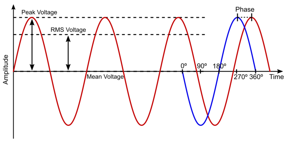
The typical waveform for an alternating current is a sine wave, when working with an AC power supply there are several indicators that must be taken into account:
Peak voltage/current: The maximum value of amplitude the wave can reach.
Frequency: The number of cycles the wave completes per second. The time it takes to complete a single cycle is called the period.
Mean voltage/current: The average value of all the points the voltage takes during one cycle. In a purely AC wave with no superimposed DC voltage, this value will be zero, because the positive and negative halves cancel each other out.
Root-mean-square voltage/current: It is defined as the square root of the mean over one cycle of the square of the instantaneous voltage. In a pure AC sinusoidal wave, its value can be calculated with: \(V_{RMS}=\frac{V_{PEAK}}{\sqrt{2}}\) It can also be defined as the equivalent DC power needed to produce the same heating effect. Despite its complicated definition, it is widely used in electrical engineering because it allows you to find the effective value of an AC voltage or current. Because of this, it is sometimes expressed as VAC.
Advantages and disadvantages of DC power supply
Direct current, in which electricity always flows in a constant direction, has the following merits and demerits:
In alternating current, the direction of the current is constantly changing. Therefore, when a capacitor or inductor is included in the circuit, for example, there is a delay or advance in the current flowing to the load in relation to the voltage behavior. However, with direct current, the voltage and the direction of the current are always constant, so the behavior of the capacitors and coils is also always constant. Therefore, in DC, there is no advance or delay in the circuit.
In alternating current (AC), the direction of the current is switched, so not all the electricity passes through the load, and some power is generated just traveling back and forth between the load and the power source. This is called reactive power, which will be discussed in later chapters. In direct current, all electricity passes through the load because the current always flows in a constant direction. Therefore, no reactive power is generated and power can be used efficiently.
Another advantage of direct current is that it can be stored by batteries or capacitors.
When a direct current flows through a circuit, it encounters various components, such as resistors, capacitors, and inductors, all of which influence its behavior. Resistors restrict current flow. There is no continuous current flow through the capacitor, while the inductor offers almost no resistance to the constant current and acts like a short circuit.
On the other hand, direct current also has its disadvantages. One of them is that it is difficult to interrupt the current. In the case of alternating current, when the voltage switches from positive to negative or negative to positive, the voltage momentarily drops to zero. If you aim for a time when the voltage is low, you can interrupt the current more safely than with a direct current.
Also, when converting DC voltage, it is necessary to convert it to AC once and then back to DC again. For this reason, DC voltage conversion equipment is larger and more costly than AC.
from PySpice.Spice.Netlist import Circuit
from PySpice.Unit import *
import matplotlib.pyplot as plt
import numpy as np

# Create a new circuit
circuit = Circuit('DC Signal')

# Define a DC voltage source
circuit.V(1, 'n1', circuit.gnd, 5@u_V)  # DC voltage of 5V

# Simulate the circuit
simulator = circuit.simulator(temperature=25, nominal_temperature=25)
analysis = simulator.operating_point()

# Extract the voltage value
voltage = float(analysis['n1'])

# Time array for plotting (0 to 10 seconds)
time = np.linspace(0, 10, 1000)
# Create an array with the DC voltage value
dc_voltage = np.full_like(time, voltage)

# Plot the DC signal
plt.figure(figsize=(10, 5))
plt.plot(time, dc_voltage, label='DC Voltage', color='blue')

# Adding labels and title
plt.title('DC Signal')
plt.xlabel('Time [s]')
plt.ylabel('Voltage [V]')
plt.axhline(0, color='black', linewidth=0.5)
plt.axvline(0, color='black', linewidth=0.5)
plt.legend()
plt.grid(True)

# Display the plot
plt.show()
Advantages and disadvantages AC power supply
Alternating current, with its cyclic positive and negative voltage, has the following advantages and disadvantages:
Compared to direct current, alternating current can be easily transformed by transformers, making it more suitable for power supply as infrastructure.
Another advantage of AC is that it is easy to shut down while power is being supplied since the timing at which the voltage drops to zero comes periodically.
It can also be used without distinguishing between positive and negative, like a household power supply (outlet), which simplifies the connection and operation of devices.
On the other hand, AC requires a higher voltage than the target voltage for the required amount of heat because the voltage value is always changing, and there are times when the voltage goes to zero. The waveform of AC voltage is sinusoidal, and the maximum voltage is √2 times the running value. Insulation performance and equipment specifications must be higher than the effective value.
Another characteristic of AC is that it is strongly affected by coils and capacitors. Coils and capacitors generate voltages that cause the current to flow in the opposite direction of the current direction, causing the current in the circuit to advance or lag.
import matplotlib.pyplot as plt
import numpy as np

# Time variable (0 to 2π for full cycle representation)
t = np.linspace(0, 2 * np.pi, 1000)

# Three-phase waveforms with 120-degree phase shift
V1 = np.sin(t)                       # Phase A
V2 = np.sin(t - 2 * np.pi / 3)       # Phase B (120-degree shift)
V3 = np.sin(t - 4 * np.pi / 3)       # Phase C (240-degree shift)

# Plot the waveforms
plt.figure(figsize=(10, 5))
plt.plot(t, V1, label='Phase A', color='red')
plt.plot(t, V2, label='Phase B', color='blue')
plt.plot(t, V3, label='Phase C', color='orange')

# Adding labels and title
plt.title('Three-phase AC')
plt.xlabel('Time [s]')
plt.ylabel('Voltage [V]')
plt.axhline(0, color='black', linewidth=0.5)
plt.axvline(0, color='black', linewidth=0.5)
plt.legend()
plt.grid(True)

# Display the plot
plt.show()
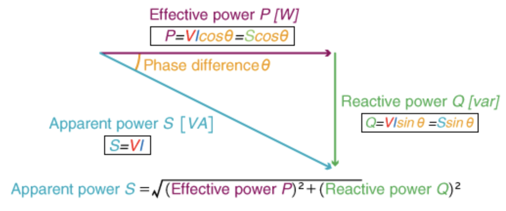
Active and reactive power in AC sources
Apparent power: The apparent power of a sinusoidal AC circuit can be calculated simply as the product of its RMS values for voltage and current. It is measured in volt-amperes (VA) or kilovolt-amps (kVA). Power is called apparent power, complex power, or total gave, and this refers to the net delivered from a source by a line. The apparent power is found by multiplying the RMS values of voltage and current, regardless of any phase relationship. The formula for apparent power is: \(S=V×I\) Where S is the apparent power, V is the RMS voltage, and I is the RMS current.
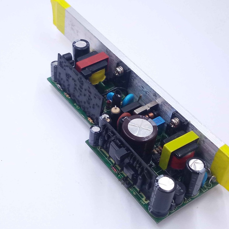
Linear AC/DC Power Supply:
A linear AC/DC power supply has a simple design. The components of a linear AC/DC power supply are transformers, rectifier and filter. By using a transformer, the alternating current (AC) input voltage is reduced to a value more suitable for the intended application. Then, the reduced AC voltage is rectified (A rectifier is an electrical device that converts alternating current (AC), which periodically reverses direction, to direct current (DC), which flows in only one direction.) and turned into a direct current (DC) voltage, which is filtered in order to further improve the waveform quality. The process inside a linear DC power supply is described as below:
Transformer: The AC voltage from the wall outlet has a high magnitude, like 110/220 V AC. Thereby, the first thing to do is transform it into a signal with a lower magnitude. This is achieved using a component called a transformer.
Rectifier: Once the AC voltage is transformed, it is then passed through a rectifier. The rectifier converts the AC voltage into pulsating DC voltage by allowing current flow in only one direction and removing the negative portion of the AC waveform.
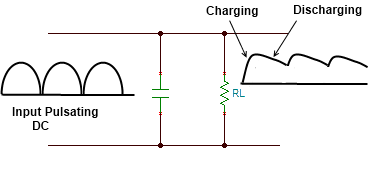
Filter: After rectifying, a filter is used to smooth out and minimize the pulsating DC voltage. Typically, due to their ability to store energy, capacitors are used in this kind of filter circuit. Regulator: To have a stable DC voltage value output, a voltage regulator is needed. It ensures a constant and stable DC voltage output, compensating for fluctuations in the load or input voltage.
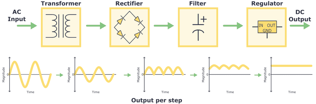
A huge limitation in a linear AC/DC power supply is the size of the transformer. Because the input voltage is transformed at the input, the necessary transformer would have to be very large and therefore very heavy.
Drawing a linear AC/DC power supply using schemdraw
The code below shows a simple linear power supply:
import matplotlib.pyplot as plt
import schemdraw
import schemdraw.elements as elm
from schemdraw import dsp

with schemdraw.Drawing() as d:
    d.push()
    elm.Line()
    tr = elm.Transformer().right().label('Transformer', loc='bot').anchor('p1')
    elm.Line().length(d.unit/3).at(tr.s1)
    elm.Line().length(d.unit/2).up()
    elm.Line().right()
    rec = elm.Rectifier().anchor('N').label('Rectifier')
    d.pop()
    elm.Gap().toy(tr.p2).label(['', 'AC IN', ''])
    elm.Line().tox(tr.p1)
    elm.Line().length(d.unit/3).at(tr.s2)
    elm.Line().length(d.unit/2).down()
    elm.Line().right()
    elm.Line().toy(rec.S)
    elm.Line().length(d.unit/8).at(rec.W).left()
    lineRec = elm.Line().length(d.unit*1.3).down()
    lineOne = elm.Line().at(rec.E).right().idot()
    line = elm.Line().idot()
    lineTwo = elm.Line().length(d.unit/3).idot()
    lineThree = dsp.Square().label('Regulator')
    lineFour = elm.Line().length(d.unit/3)
    lineFive = elm.Line().length(d.unit/2).idot()
    elm.Gap().toy(lineRec.end).label(['+', 'DC OUT', '–'])
    lineFiveEnd = elm.Line().length(d.unit/2).left().dot()
    lineThreeEnd = elm.Line().tox(lineThree.S).dot()
    lineTwoEnd = elm.Line().tox(lineTwo.start).dot()
    lineEnd = elm.Line().tox(line.start).dot()
    lineOneEnd = elm.Line().tox(lineOne.start)
    elm.Line().tox(lineRec.end)
    elm.Capacitor().endpoints(lineOne.end,lineOneEnd.start).label('Filter')
    elm.Capacitor().endpoints(lineTwo.start,lineEnd.start).label('C1')
    elm.Line().endpoints(lineTwoEnd.start,lineThree.S)
    elm.Capacitor().endpoints(lineFive.start,lineFiveEnd.end).label('C2')
plt.show()
Switching AC/DC Power Supply:
New design methodology has been developed to solve many of the problems associated with linear or traditional AC/DC power supply design, including transformer size and voltage regulation. Switching power supplies are now possible thanks to the evolution of semiconductor technology, especially thanks to the creation of high-power MOSFET transistors, which can switch on and off very quickly and efficiently, even if large voltages and currents are present. A switching AC/DC power supply enables the creation of more efficient power converters, which no longer dissipate the excess power.
In switching AC power supplies, the input voltage is no longer reduced; rather, it is rectified and filtered at the input. Then the DC voltage goes through a chopper, which converts the voltage into a high-frequency pulse train. Finally, the wave goes through another rectifier and filter, which converts it back to direct current (DC) and eliminates any remaining alternating current (AC) component that may be present before reaching the output. The process is shown as below:
Bridge rectifier—AC main to DC pulse: Normally, we will find this rectifier circuit at the input side of the switching power supply. Then, the DC pulse passes through to an RF switch circuit.
Half-wave rectifier for RF AC Signal: In a switching power supply, the input DC signal will be switched with a high-frequency RF signal. Then, the step-down transformer transforms it into low-voltage AC. Next, it flows through a half-wave rectifier to be rectified into a DC pulse. The heart of every switching power supply is the RF Regulator. Also known as the “Switching Regulator.”
Full-wave rectifier using Center Tap Transformer: This is a step up from a half-wave rectifier. And it uses the center tap of the transformer’s secondary coil. When operating at high frequencies, the transformer’s inductor is able to transfer more power without reaching saturation, which means the core can become smaller and smaller. Therefore, the transformer used in switching AC/DC power supplies to reduce the voltage amplitude to the intended value can be a fraction of the size of the transformer needed for a linear AC/DC power supply.
Full-wave bridge rectifier after a Step-down transformer: Or we can instead use two more diodes.
Output Rectifier and Filter: Converts the AC output from the transformer back to DC and smooths it. Switching AC/DC power converters can generate a significant amount of noise in the system, which must be treated to ensure it is not present at the output. This creates a need for more complex control circuitry, which in turn adds complexity to the design. Nevertheless, these filters are made up of components that can be easily integrated, so it does not affect the size of the power supply significantly.
Although there are many different switching circuits. But the most common one used is PWM (Pulse Width Modulation). The figure is a basic block diagram of the PWM switching regulator. It maintains the voltage level in a closed-loop form:
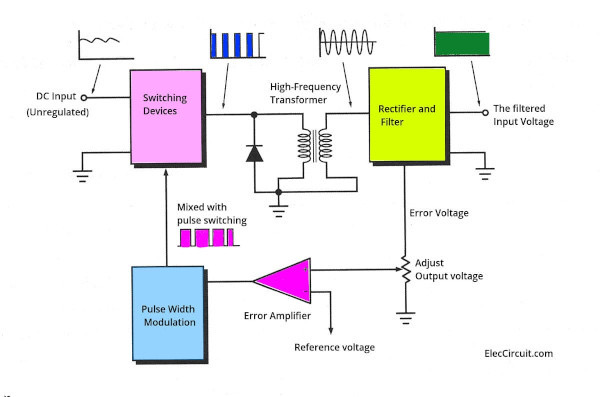
Smaller transformers and increased voltage regulator efficiency in switching AC/DC power supplies are the reason why we can now convert a 220V¬RMS AC voltage to a 5V DC voltage with a power converter that can fit in the palm of your hand.
1. Transformer
Function: Steps up or steps down the AC voltage to match the needs of the circuit
Working Principle:
Uses electromagnetic induction to change voltage without altering the frequency
Often includes a center tap in full-wave rectifiers to allow more efficient conversion
Benefits: Electrical isolation from the power source
Voltage adaptation for safety and compatibility
2. Rectifier Circuit
Function:
Converts AC voltage to pulsating DC voltage
Common Components:
Diodes for uncontrolled rectification
SCRs (Thyristors) or other controlled switches for adjustable output
Typical Types:
Half-Wave Rectifier: Uses only one half-cycle of AC; simple but inefficient
Full-Wave Rectifier (Center Tap or Bridge): Uses both half-cycles for higher efficiency and lower ripple
Notes:
A diode bridge uses four diodes
In controlled rectifiers, firing angle can be adjusted to regulate output voltage
3. Filter (Capacitor / Inductor)
Function: Smooths out fluctuations (ripple) in the rectified DC signal
Main Filtering Components:
Capacitor: Role: Stores and releases charge to fill voltage gaps
Effect: Significantly reduces voltage ripple
Placement: Connected in parallel with the load
Inductor: Role: Resists rapid changes in current
Effect: Smooths the DC current flow
Placement: Typically in series with the load or part of LC/π filters
Combo: Using both capacitor and inductor in LC or π-filter configurations results in better DC quality
4. Voltage Regulator
Role:
Stabilizes the output DC voltage to protect the load and reduce residual fluctuations.
Application: After filtering, the voltage may still fluctuate slightly or be slightly higher than required. Regulators (such as 7805 for 5V, 7812 for 12V, etc.) are responsible for keeping the DC output at a certain and stable value. In more complex systems, switching regulators are also used.
An alternating current (AC) power supply can either be single-phase or three-phase:
A three-phase power supply is composed of three conductors, called lines, which each carry an alternating current (AC) of the same frequency and voltage amplitude, but with a relative phase difference of 120°, or one-third of a cycle. These systems are the most efficient at delivering large amounts of power, and are therefore used for delivering electricity from generating facilities to homes and businesses all around the world. An example of this was provided above.
A single-phase power supply is the preferred method to supply current to individual homes or offices, so as to distribute the load evenly between lines. In this case, the current flows from the power line through the load, then back through the neutral wire. This is the type of supply found in most installations, except large industrial or commercial buildings. Single-phase systems cannot transfer as much power to loads and are more prone to power failures, but single-phase power also allows use of much simpler networks and devices.
There are two configurations for the transmission of power through a three-phase power supply: delta (Δ) and wye (Y) configurations, also referred to as triangle and star configurations, respectively. The main difference between these two configurations is the ability to add a neutral wire. Delta connections offer greater reliability, but Y connections can supply two different voltages: phase voltage, which is the single-phase voltage supplied to homes, and line voltage, for powering larger loads. The Delta configuration has the 3 phases connected like in a triangle. They don’t normally have a neutral cable. In Delta configuration, the phase voltage is equal to the line voltage whereas in Y configuration, the phase voltage is the line voltage divided by root 3. Wye configurations are typically used for systems where a neutral is required, such as in distribution networks for residential or commercial buildings, because they allow for both 120V and 240V outputs; Delta configurations are often used in industrial settings where high power is required, and a neutral is not necessary, such as in motors and heavy machinery.
The image below shows how a Y and Delta configurations wires are attached:
As mentioned before, three-phase power is not only used for transportation, but is also used to power large loads, such as electric motors or charging large batteries. This is because the parallel application of power in three-phase systems can transfer much more energy to a load, and can do so more evenly, due to the overlapping of the three phases. For example, when charging an electric vehicle (EV), the amount of power you can transfer to the battery determines how fast it charges. Single-phase chargers are plugged into the alternating current (AC) mains and converted to direct current (DC) by the car’s internal AC/DC power converter (also called an on-board charger). These chargers, are limited in power by the grid and the AC socket.
The image below shows the power transfered in Single-Phase and Three-Phase systems:
This examples shows the computation of the voltage for the Y and Delta configurations. Lets use an 220 V / 50 Hz electric network. The phase voltages in Y configuration are dephased of $\frac{2\pi}{3}$ :
\(V_{L1-N} = V_{pp} cos(𝜔t)\) \(V_{L2-N} = V_{pp} cos(𝜔t-\frac{2\pi}{3})\) \(V_{L3-N} = V_{pp} cos(𝜔t-\frac{4\pi}{3})\)
We rewrite them in complex notation: \(V_{L1-N} = V_{pp} e^{jwt}\) \(V_{L2-N} = V_{pp} e^{j(wt-\frac{2\pi}{3})}\) \(V_{L3-N} = V_{pp} e^{j(wt-\frac{4\pi}{3})}\)
From these expressions, we compute the voltage in delta configuration using trigonometric identities :
\(V_{L1-L2} = V_{L1} \sqrt{3}\ e^{j\frac{\pi}{6}}\) \(V_{L2-L3} = V_{L2} \sqrt{3}\ e^{j\frac{\pi}{6}}\) \(V_{L3-L1} = V_{L3} \sqrt{3}\ e^{j\frac{\pi}{6}}\)
In comparison to the Y configuration, the voltages in delta configuration are magnified by a factor $/sqrt{3}$ and dephased of $\frac{\pi}{6}$ .
Finally we rewrite them in temporal notation:
\(V_{L1-L2} = V_{pp} \sqrt{3} cos(𝜔t+\frac{\pi}{6})\) \(V_{L2-L3} = V_{pp} \sqrt{3} cos(𝜔t-\frac{\pi}{2})\) \(V_{L3-L1} = V_{pp} \sqrt{3} cos(𝜔t-\frac{7\pi}{6})\)
Now we plot the waveforms:
import math
import numpy as np
import matplotlib.pyplot as plt
from PySpice.Unit import *

frequency = 50@u_Hz
w = frequency.pulsation
period = frequency.period
rms_mono = 220
amplitude_mono = rms_mono * math.sqrt(2)

t = np.linspace(0, 3*float(period), 1000)

##Y configuration
L1 = amplitude_mono * np.cos(t*w) ##phase one
L2 = amplitude_mono * np.cos(t*w - 2*math.pi/3) ##phase two
L3 = amplitude_mono * np.cos(t*w - 4*math.pi/3) ##phase three

rms_tri = math.sqrt(3) * rms_mono
amplitude_tri = rms_tri * math.sqrt(2)

##Delta configuration
L12 = amplitude_tri * np.cos(t*w + math.pi/6)
L23 = amplitude_tri * np.cos(t*w - math.pi/2)
L31 = amplitude_tri * np.cos(t*w - 7*math.pi/6)

figure, ax = plt.subplots(figsize=(20, 10))
ax.plot(
    t, L1, t, L2, t, L3,
    t, L12, t, L23, t, L31,
    # t, L1-L2, t, L2-L3, t, L3-L1,
)
ax.grid()
ax.set_title('Three-phase electric power: Y and Delta configurations (220V Mono/400V Tri 50Hz Iran)')
ax.legend(
    ('L1-N', 'L2-N', 'L3-N',
     'L1-L2', 'L2-L3', 'L3-L1'),
    loc=(.7,.5),
)
ax.set_xlabel('t [s]')
ax.set_ylabel('[V]')
ax.axhline(y=rms_mono, color='blue')
ax.axhline(y=-rms_mono, color='blue')
ax.axhline(y=rms_tri, color='blue')
ax.axhline(y=-rms_tri, color='blue')

plt.show()
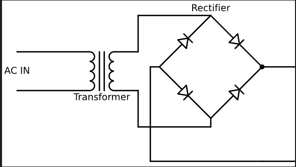
A half-wave rectifier converts AC to DC by blocking one half of the waveform, using a single diode, and is less efficient than a full-wave rectifier. A full-wave rectifier, such as the full bridge rectifier with four diodes, converts the entire waveform to DC, providing a smoother output.
Power diodes can be used individually as below or connected together to produce a variety of rectifier circuits
In many applications, we reduce the peak voltage using a transformer before applying it to a half-wave rectifier.
During the positive half-cycle of the AC sine wave, the forward-biased diode allows current to flow, making the output voltage equal to the supply voltage minus the diode’s forward voltage. In the negative half-cycle, the reverse-biased diode blocks current, resulting in an output voltage of zero.
The DC side of the circuit is unidirectional, with the load resistor receiving an irregular voltage waveform comprising positive and zero volts. This voltage is equivalent to $ 0.318 * V_\text{max} $ or $ 0.45 * V_\text{rms} $ of the input sinusoidal waveform.
DC output value calculation
\[V_{\text{avg}} = \frac{1}{T} \int_{0}^{T} v(t) \, dt\]For a half-wave rectified sinusoidal waveform, we need to consider the average over one period, but since the waveform is rectified, it’s zero for half the period. Thus, we compute the average over the non-zero half-cycle and then use the formula for the full period.
The waveform $ v(t) = V_{\text{max}} \sin(\omega t) $ for $0 \leq t < T/2$ and zero for $ T/2 \leq t < T $.
The average value over the period is:
\[V_{\text{avg}} = \frac{1}{T} \int_{0}^{T} v(t) \, dt\]Since $ v(t) = V_{\text{max}} \sin(\omega t) $ from $0$ to $T/2$ and $0$ from $T/2$ to $T$:
\[V_{\text{avg}} = \frac{1}{T} \left( \int_{0}^{T/2} V_{\text{max}} \sin(\omega t) \, dt \right)\]Compute the integral:
\[\int_{0}^{T/2} V_{\text{max}} \sin(\omega t) \, dt = \frac{V_{\text{max}}}{\omega} \left[ -\cos(\omega t) \right]_{0}^{T/2}\]Substituting the limits:
\[\frac{V_{\text{max}}}{\omega} \left[ -\cos\left(\frac{\omega T}{2}\right) + \cos(0) \right]\]Since $\cos\left(\frac{\omega T}{2}\right) = \cos(\pi) = -1$ and $\cos(0) = 1$:
\[\frac{V_{\text{max}}}{\omega} \left[ -(-1) + 1 \right] = \frac{V_{\text{max}}}{\omega} \cdot 2\]Therefore:
\[\frac{1}{T} \cdot \frac{V_{\text{max}} \cdot 2}{\omega}\]Since $\omega = \frac{2\pi}{T}$:
\[\frac{1}{T} \cdot \frac{2 V_{\text{max}} T}{2 \pi} = \frac{2 V_{\text{max}}}{2 \pi} = \frac{V_{\text{max}}}{\pi}\]So, the correct average value $ V_{\text{avg}} $ is:
\[V_{\text{DC}} =V_{\text{avg}} = \frac{V_{\text{max}}}{\pi}=0.318V_{\text{max}}\]also we write $ V_{\text{rms}} $ in terms of $ V_{\text{max}} $:
\[V_{\text{rms}} = \frac{V_{\text{max}}}{\sqrt{2}}\]Express $ V_{\text{max}} $ in terms of $ V_{\text{DC}} $:
Given $ V_{\text{DC}} = \frac{V_{\text{max}}}{\pi} $,
\[V_{\text{max}} = \pi \times V_{\text{DC}}\]Substitute $ V_{\text{max}} $ into the $ V_{\text{rms}} $ formula:
\[V_{\text{rms}} = \frac{\pi \times V_{\text{DC}}}{\sqrt{2}}\]Simplify the expression:
\[V_{\text{rms}} = \pi \times \frac{V_{\text{DC}}}{\sqrt{2}}\]So,
\[V_{\text{DC}} \approx 0.45 \times V_{\text{rms}}\]Reminder: To find $ V_{\text{rms}} $ of the input sinusoidal signal over one period, and then relate it to $ V_{\text{DC}} $, we should calculate the RMS value for the entire period of the input signal.
RMS value of the input sinusoidal signal:
The input sinusoidal signal $ v(t) = V_{\text{max}} \sin(\omega t) $ over one period $ T $ has the RMS value:
\[V_{\text{rms}} = \sqrt{\frac{1}{T} \int_0^T \left(V_{\text{max}} \sin(\omega t)\right)^2 \, dt}\] \[V_{\text{rms}} = V_{\text{max}} \sqrt{\frac{1}{T} \int_0^T \sin^2(\omega t) \, dt}\]Using the identity $ \sin^2(x) = \frac{1 - \cos(2x)}{2} $:
\[\sin^2(\omega t) = \frac{1 - \cos(2\omega t)}{2}\]Thus,
\[V_{\text{rms}} = V_{\text{max}} \sqrt{\frac{1}{T} \int_0^T \frac{1 - \cos(2\omega t)}{2} \, dt}\] \[V_{\text{rms}} = V_{\text{max}} \sqrt{\frac{1}{T} \cdot \frac{1}{2} \int_0^T (1 - \cos(2\omega t)) \, dt}\]The integral of $ 1 $ over $ 0 $ to $ T $ is $ T $, and the integral of $ \cos(2\omega t) $ over one period $ T $ is zero:
\[\int_0^T 1 \, dt = T\] \[\int_0^T \cos(2\omega t) \, dt = 0\]So,
\[V_{\text{rms}} = \frac{V_{\text{max}}}{\sqrt{2}}\]Full Wave Rectifier
Power diodes can be connected to form a full wave rectifier, converting AC voltage into DC voltage for power supplies. This rectifier uses four diodes to convert both halves of each AC waveform cycle into a DC signal. While smoothing capacitors can reduce ripple for low-power applications, a full wave rectifier is more efficient for higher power needs, utilizing every half-cycle of the input voltage.
How its work
The Positive Half-cycle
The Negative Half-cycle
Advantages and Circuit Operation
A full wave rectifier produces a higher average DC output voltage with less ripple compared to a half wave rectifier, resulting in a smoother output waveform. Such as Half Wave Rectifier, can reach to:
A full-wave rectifier converts the entire AC waveform into DC, providing a smoother and more efficient output compared to a half-wave rectifier. It utilizes four diodes to rectify both halves of the AC cycle, resulting in a higher average DC output with reduced ripple.
Power diodes can be configured into various rectifier circuits. A common design is the full-wave rectifier, using a center-tapped transformer and two diodes to handle both half-cycles of the input waveform. This configuration doubles the frequency of the output signal, resulting in a smoother DC output.
DC Output Value Calculation
For a full-wave rectifier, the average DC output voltage $V_{\text{DC}}$ is given by:
\[V_{\text{DC}} = \frac{2 V_{\text{max}}}{\pi}\]where $ V_{\text{max}} $ is the peak value of the AC signal. This result shows that the DC output voltage is higher and smoother compared to a half-wave rectifier.
The circuit uses two diodes and a center-tapped transformer, allowing each diode to conduct during opposite half-cycles. This configuration doubles the output frequency, making the full wave rectifier 100% efficient. The consistent current direction through the load resistor during both half-cycles ensures a continuous DC output.
Capacitors smooth the full-wave rectifier output, reducing peak-to-peak ripple for a more stable voltage.
Ripple is the residual AC component in the output of a half-wave rectifier that causes the DC waveform to pulsate. The ripple factor $ \gamma $ quantifies this unwanted AC component and is obtained as:
\[\gamma = \frac{\text{RMS value of the AC component}}{\text{DC component value}} = \frac{V_{r(\text{rms})}}{V_{dc}}.\] \[\gamma = \sqrt{\frac{V_{rms}^2}{V_{dc}^2} - 1}.\]Proof: Here, $ V_{r(\text{rms})} $ represents the RMS value of the AC component, and $ V_{dc} $ is the DC component of the output.
To determine $ V_{r(\text{rms})} $, we start by expressing the output voltage of the half-wave rectifier as:
\[V_o(t) = V_{ac} + V_{dc},\]where $ V_{ac} $ is the AC component remaining after rectification. The RMS value of the AC component can be calculated using:
\[V_{r(\text{rms})} = \left( \frac{1}{T} \int_0^T V_{ac}^2 \, dt \right)^{1/2}.\]We can also write $ V_{r(\text{rms})} $ as:
\[V_{r(\text{rms})}^2 = \frac{1}{T} \int_0^T (V_o - V_{dc})^2 \, dt.\]Expanding the square and integrating, we get:
\[V_{r(\text{rms})}^2 = \frac{1}{T} \int_0^T (V_o^2 - 2V_o V_{dc} + V_{dc}^2) \, dt.\]This simplifies to:
\[V_{r(\text{rms})}^2 = \frac{1}{T} \int_0^T V_o^2 \, dt - \frac{2V_{dc}}{T} \int_0^T V_o \, dt + V_{dc}^2.\]Since $ \frac{1}{T} \int_0^T V_o \, dt = V_{dc} $, we have:
\[V_{r(\text{rms})}^2 = V_{rms}^2 - V_{dc}^2,\]where $ V_{rms} $ is the RMS value of the entire voltage signal.
Therefore, the ripple factor $ \gamma $ can be written as:
\[\gamma = \sqrt{\frac{V_{rms}^2}{V_{dc}^2} - 1}.\]Substituting the values for $ V_{dc} $ and $ V_{rms} $, we find:
\[\gamma = \sqrt{\frac{V_m^2 / 2 \cdot \pi}{V_m / \pi}^2 - 1} = \sqrt{\left(\frac{\pi}{2}\right)^2 - 1} \approx 1.21.\]Ripple Factor of a Full-Wave Rectifier
The ripple factor ($ \gamma $) for a full-wave rectifier is defined as:
\[\gamma = \frac{V_{r(\text{rms})}}{V_{dc}} = \sqrt{\frac{V_{rms}^2}{V_{dc}^2} - 1},\]where $ V_{r(\text{rms})} $ is the RMS value of the AC component, and $ V_{dc} $ is the DC component. For a full-wave rectifier, the ripple factor simplifies to:
\[\gamma = \sqrt{\left(\frac{\pi}{2\sqrt{2}}\right)^2 - 1} \approx 0.48.\]A voltage multiplier is an electrical circuit that converts AC electrical power from a lower voltage to a higher DC voltage, typically using a network of capacitors and diodes. Voltage multipliers can be used to generate a few volts for electronic appliances, to millions of volts.
Example $ V_o $ of four times the peak of the AC input voltage $ V_i $
After rectification, the DC output can be further stabilized using regulators, which are primarily of two types:
Linear Regulators: These provide a stable output voltage by using a linear pass element to drop excess voltage. They are simple and offer low noise but are less efficient, especially with large voltage drops.
Switching Regulators: These use high-frequency switching elements to convert input voltage to a desired output voltage with higher efficiency. They are more complex but provide better efficiency and can step up, step down, or invert the voltage.
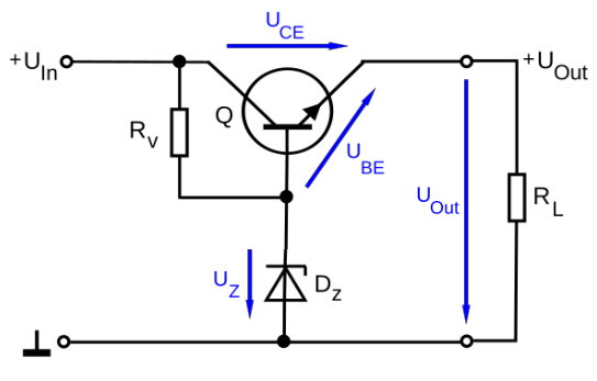
A simple transistor regulator maintains a relatively constant output voltage (Uout) despite changes in input voltage (Uin) and load resistance (RL), provided Uin exceeds Uout sufficiently and the transistor’s power capacity isn’t exceeded. The stabilizer’s output voltage equals the Zener diode voltage minus the transistor’s base-emitter voltage (UZ − UBE), with UBE typically around 0.7 V for silicon transistors. If Uout drops due to external factors, UBE increases, activating the transistor further to boost the load voltage. Rv supplies bias current to both the Zener diode and transistor, with its value affecting input voltage requirements and regulator efficiency. Lower Rv values increase diode power dissipation and worsen regulator performance.
Regulator with a differential amplifier
The stability of the output voltage can be enhanced by using a differential amplifier, such as an operational amplifier. It adjusts the transistor current based on input voltage discrepancies, allowing for an adjustable output voltage via a voltage divider.

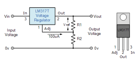
Example of linear regulator is LM317: Adjustable 1.5 A positive voltage regulator (1.25 V-37 V)


A relay circuit consists of three key components: switches, a relay coil, and a diode. The switches ensure reliable electrical contact without bounce, while the relay coil controls the switching between open and closed states. The diode provides transient voltage suppression, protecting the switching circuitry from voltage spikes caused by the relay’s activation and deactivation.

import matplotlib.pyplot as plt
import schemdraw
import schemdraw.elements as elm
from schemdraw import dsp

with schemdraw.Drawing() as d:
    d.push()
    elm.Line()
    tr = elm.Transformer().right().label('Transformer', loc='bot').anchor('p1')
    elm.Line().length(d.unit/3).at(tr.s1)
    elm.Line().length(d.unit/2).up()
    elm.Line().right()
    rec = elm.Rectifier().anchor('N').label('Rectifier')
    d.pop()
    elm.Gap().toy(tr.p2).label(['', 'AC IN', ''])
    elm.Line().tox(tr.p1)
    elm.Line().length(d.unit/3).at(tr.s2)
    elm.Line().length(d.unit/2).down()
    elm.Line().right()
    elm.Line().toy(rec.S)
    elm.Line().length(d.unit/8).at(rec.W).left()
    lineRec = elm.Line().length(d.unit*1.3).down()
    lineOne = elm.Line().at(rec.E).right().idot()
    line = elm.Line().idot()
    lineTwo = elm.Line().length(d.unit/3)
    lineThree = dsp.Square().label('Regulator')
    lineFour = elm.Line().length(d.unit/3)
    lineFive = elm.Line().length(d.unit/2)
    elm.Gap().toy(lineRec.end).label(['+', 'DC OUT', '–'])
    lineFiveEnd = elm.Line().length(d.unit/2).left()
    lineThreeEnd = elm.Line().tox(lineThree.S)
    lineTwoEnd = elm.Line().tox(lineTwo.start)
    lineEnd = elm.Line().tox(line.start).dot()
    lineOneEnd = elm.Line().tox(lineOne.start)
    elm.Line().tox(lineRec.end)
    elm.Capacitor().endpoints(lineOne.end,lineOneEnd.start).label('Filter')

    elm.Line().endpoints(lineTwoEnd.start,lineThree.S)


plt.show()
AC to DC converters are not only fundamental in small electronic circuits but also play a vital role in many industrial systems. Their ability to convert alternating current (AC) to direct current (DC) makes them essential in power systems, manufacturing processes, and modern technologies.
Industrial Applications
Consumer Electronics and Telecommunications: Nearly all modern electronic devices – from computers to smartphones – require DC voltage, which is supplied through AC/DC power converters.
Automotive Industry: Electric and hybrid vehicles use AC to DC converters for charging batteries and powering internal electronic systems.
Control Systems and Automation: In industrial automation, devices like PLCs, sensors, and motor drives operate on DC power. Converters provide stable voltage for these control systems.
Industrial Power Supplies: Switch-mode power supplies (SMPS) in industrial applications rely on efficient AC to DC conversion for high-performance and energy-saving operations.
Technological Advancements
Recent technological developments have significantly improved the performance of AC to DC converters:
Advanced Semiconductor Materials (SiC, GaN) : These materials are used to build faster and more efficient power devices with lower losses.
High-Efficiency and Compact Designs : Modern converters are designed to be smaller, lighter, and more efficient, using advanced topologies and control methods.
Digital Control and Smart Features : Integration of microcontrollers and digital signal processing allows for smarter and more precise regulation of output voltage and current.
While AC to DC converters are essential in various applications, their design and operation face several challenges. These issues range from technical and design-related problems to efficiency concerns and safety risks.
Technical Challenges
Ripple Voltage:
Even after rectification, the output DC voltage is not completely smooth. Ripple can cause instability or malfunction in sensitive electronic circuits.
Voltage Drop in Diodes:
Every diode has a forward voltage drop (typically ~0.7V for silicon diodes), which reduces the overall efficiency, especially in low-voltage applications.
Heat Loss:
Power components such as regulators and diodes produce heat, and without proper thermal management, performance may degrade or components may fail.
Design and Economic Challenges
Size and Weight at High Power Levels:
High-power converters require large components like transformers or capacitors, increasing the size and weight of the system.
Cost of Advanced Components:
While using modern semiconductors like GaN or SiC improves performance, it significantly raises the design and production costs.
Complex Control Requirements:
Smart or digital AC/DC converters often require precise control algorithms and microcontrollers, making the system more complex to design and maintain.
The conversion of alternating current to direct current represents a cornerstone of modern electrical engineering, enabling the operation of countless electronic devices and industrial systems. This research has systematically examined the fundamental principles, operational mechanisms, and practical applications of AC to DC power conversion.
The comprehensive analysis revealed distinct advantages and disadvantages of both AC and DC power supplies, highlighting their complementary roles in electrical systems. The investigation of linear versus switching conversion methods demonstrated the superior practicality of switching techniques, particularly in terms of transformer size optimization and overall efficiency.
Furthermore, the exploration of three-phase power systems, including Y and Delta configurations, underscored their significant advantage in power transmission capacity compared to single-phase systems. The detailed examination of rectifier circuits, voltage regulation techniques, and component selection criteria provides valuable insights for practical implementation.
Looking forward, the field of AC to DC conversion continues to evolve with emerging technologies and innovative approaches. Future research directions should focus on developing advanced semiconductor materials, intelligent control algorithms, and integrated power management solutions to address ongoing challenges in efficiency, thermal management, and system miniaturization.
In essence, this research contributes to a deeper understanding of power conversion technologies and their critical role in bridging the gap between AC power distribution networks and DC-powered applications, ultimately supporting the advancement of more efficient and sustainable electrical systems.
https://www.sciencefacts.net/direct-current.html https://www.monolithicpower.com/en/learning/resources/ac-dc-power-supply-basics https://www.matsusada.com/column/dc_and_ac.html https://eshop.se.com/in/blog/post/difference-between-active-power-reactive-power-and-apparent-power.html https://en.wikipedia.org/wiki/Rectifier https://pyspice.fabrice-salvaire.fr/releases/v1.4/examples/electricity/three-phase.html https://www.build-electronic-circuits.com/linear-power-supply/ https://www.eleccircuit.com/what-switching-power-supply-how-does-it-work/ https://youtu.be/jsBn2r94BDA https://youtu.be/JXJaRPXPwjQ https://www.rohm.com/electronics-basics/ac-dc-converters/acdc_what1
*اصلاح فرمت عکس ها- فارسی -انگلیسی - ادرس دهی -فهم مطالب*\