
Single-class anomaly detection based on implicit convex hull and ensemble learning

🎓 M.Sc. in Computer Engineering (2022–2025)
🤖 Specialization: Artificial Intelligence and Robotics
📊 Research Area: Anomaly Detection and Decentralized Models
🏆 Graduation Grade: Excellent (19.5)
🎓 Supervisor’s Message
I sincerely congratulate Yousof Ghalenoei on graduating with an excellent grade (19.5). His effort, perseverance, and creativity in the fields of anomaly detection and decentralized learning are a valuable example for other students. I wish him the best of success in his research and professional future.
Dr. Hadi Sadeghi Yazdi, Supervisor
📬 Contact Information
Abstract
In this research, a novel framework for anomaly detection is proposed, which is based on one-class classification and the implicit representation of a convex hull of the normal data region. The main idea is to estimate the decision boundary implicitly through elastic net regularization; the simultaneous combination of $\ell_1$ and $\ell_2$ in the elastic net leads, on the one hand, to sparsity and effective feature selection, and on the other hand provides numerical stability and a grouping effect among correlated features. To improve accuracy and reduce the bias caused by data imbalance, we employ ensemble learning based on sampling and random subspaces. The optimization problem is solved using proximal gradient methods and AMP algorithms. To overcome AMP’s convergence limitations, its advanced version, KAMP, is used, which combines Kalman filter ideas with AMP to achieve more stable and faster convergence under noisy conditions and ill-conditioned matrices. Furthermore, its distributed variant, DKAMP, guarantees scalability and efficiency in large networks by dividing the measurement matrix among nodes and exchanging small messages through diverse graph topologies.
The proposed framework is evaluated on diverse benchmark datasets and compared with prominent methods such as OCSVM, SVDD, LOF, IF, and EE. The results show that the proposed model significantly improves not only the arithmetic and geometric mean scores but also metrics such as precision, accuracy, recall, F1, and kappa, providing stable and reliable performance across different data structures and distributions. Thus, the combination of the implicit convex hull, elastic net regularization, AMP, KAMP, DKAMP, and ensemble learning delivers a coherent, scalable, and robust framework for anomaly detection in real-world scenarios and complex datasets.
Problem Definition
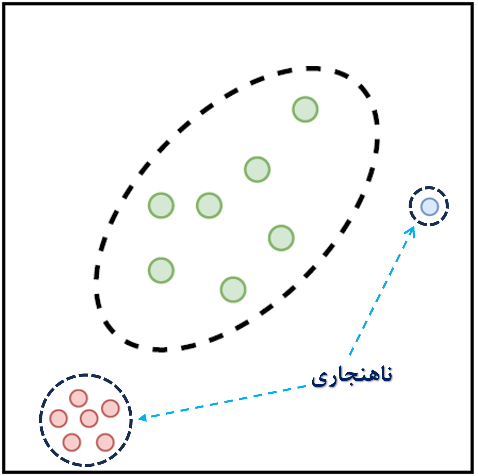
Anomalies are patterns in data that do not conform to a well-defined notion of normal behavior. Anomaly detection refers to the problem of finding patterns in data that deviate from expected normal behavior. These mismatched patterns are commonly referred to as anomalies, outliers, inconsistent observations, and exceptions in various contexts. Among these, anomalies and outliers are two terms frequently used in anomaly detection and are sometimes used interchangeably. The importance of anomaly detection lies in the fact that anomalies often translate into critical information for necessary actions. Many machine learning systems assume that their training experience represents the test experience; however, in the real world, this assumption is incorrect. “New” or “anomalous” data, not present in the training set, can lead to reduced prediction accuracy and safety concerns. For example, autonomous driving systems must alert humans when encountering unknown conditions or objects they have not been trained on, and an anomalous MRI scan may indicate the presence of malignant tumors.
Another related concept is novelty detection, which aims to identify previously unseen (emerging, new) patterns in data. The difference between novel patterns and anomalies is that novel patterns may often be incorporated into the normal model after detection.
Moreover, in real-world scenarios, due to practical applications in companies or industries, generated data often have imbalanced distributions. For example, tasks such as disease detection, biological disorder analysis, natural disaster prediction, anomaly detection, fraud detection, and biometric applications such as authentication involve imbalanced datasets. In 1969, Grubbs was the first to define an anomaly as: “an outlying observation that clearly deviates from other members of the sample in which it occurs.” Thus, a simple approach to anomaly detection is to define a region representing normal behavior and declare any observation outside this region as an anomaly. However, various factors turn this seemingly simple approach into a major challenge. For instance, in machine learning, it is typically assumed that the number of samples in each studied class is approximately equal. In contrast, in anomaly detection problems that usually involve imbalanced data, the use of conventional classification methods (binary or multiclass) leads to bias toward the class or classes with more samples. In such situations, where modeling and detecting minority class samples is very difficult, using a one-class classifier (OCC) is a suitable approach for detecting abnormal data relative to the known (majority) class data. OCC (Figure 1) is a special case of multiclass classification, where the observed data during training belong only to one positive class, while the negative class either does not exist, is poorly sampled, or is not clearly defined. OCC is also studied in specific problems such as noisy data, feature selection, and dimensionality reduction in big data.
Anomaly detection using Convex Analysis (CA) within the framework of one-class classification (OCC) is an important technique for identifying “new” or “anomalous” samples, with wide-ranging applications. Convex analysis uses techniques for determining geometric boundaries of the target set.
Convex analysis (convex hull), in addition to its high computational complexity $\mathcal{O}(n^{\lfloor\frac{p}{2}\rfloor})$ and lack of scalability, is less effective when dealing with non-convex sets. Furthermore, many convex hull-based methods perform poorly when facing multimodal and non-convex data. On the other hand, most OCC methods result in a quadratic programming problem, the solution of which becomes highly costly at large scales. To overcome these limitations, in recent years, Approximate Message Passing (AMP) algorithms have emerged as efficient iterative methods for solving signal reconstruction problems. AMP offers fast convergence, but its convergence guarantees hold only under ideal conditions, such as sub-Gaussian random matrices. To overcome this limitation, an extended version called Kalman-AMP (KAMP) has been introduced, which combines Kalman filter ideas with AMP to improve stability and convergence in noisy and ill-conditioned scenarios. Moreover, to enhance scalability, the decentralized version of this algorithm, called Distributed KAMP (DKAMP), has been developed. In this version, the measurement matrix is distributed among the nodes of a graph, and each node runs a local KAMP algorithm and exchanges information with neighbors (using strategies such as random communication) to reach a collective and robust estimate.
This design enables the practical application of AMP- and KAMP-based methods in large and dynamic graph environments, making them resilient to noise and complex data structures. In summary, the problem addressed in this research can be stated as follows: the design and development of a one-class classification framework based on an implicit convex hull boundary, which, through the use of efficient iterative algorithms (AMP) and their extensions (KAMP and DKAMP), can overcome the challenges of convex hull computation, scalability, and stability under noisy and ill-conditioned data.
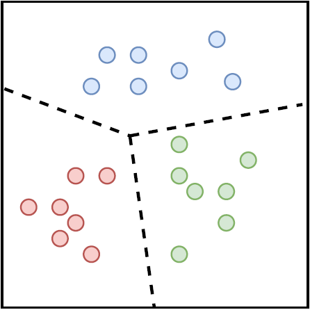
(a) Multi-class Classification
(b) One-class Classification
Figure 1: Difference between one-class and multi-class classifiers
A Part of the Reviewed Literature
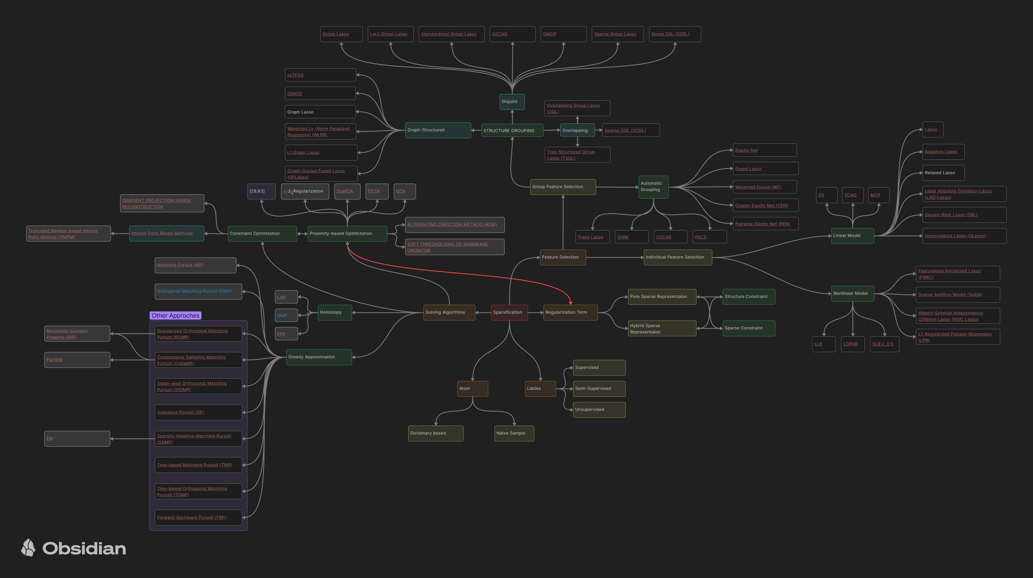
A part of the reviewed literature related to sparse methods
Theoretical Foundations
Introduction to Proximal Algorithms
Proximal Algorithms are a class of optimization methods for solving convex problems. Similar to the role of Newton’s method in smooth and small-scale problems, these algorithms are considered standard tools for nonsmooth, constrained, large-scale, and distributed problems.
The main advantage of these methods is their ability to handle large datasets and high-dimensional problems. The fundamental operation in these algorithms is computing the proximal operator, which is equivalent to solving a small convex optimization problem. These subproblems often have closed-form solutions or can be solved with simple and fast methods.
1.1 Definition
If $f: \mathbb{R}^n \to \mathbb{R} \cup {+\infty}$ is a convex function, its proximal operator is defined as follows:
\(\text{prox}_{\lambda f}(v) = \arg\min_x \Big( f(x) + \tfrac{1}{2\lambda}\|x - v\|_2^2 \Big)\) This definition ensures that for any vector $v$ there exists a unique solution.
1.2 Interpretations
- Geometric View: The proximal operator moves the point $v$ toward the minimizer set of the function $f$, establishing a trade-off between staying close to $v$ and reducing the value of $f(x)$.
- Relation to Projection: If $f$ is the indicator function of a convex set, the proximal operator is exactly the projection onto that set.
- Dynamic View: The proximal operator can be seen as a step in iterative dynamic methods that follow the optimal path.
1.3 Examples
Some important examples of proximal operators that frequently appear in applications:
- $\ell_2$ function: its proximal operator is simply a scaling of the vector.
- $\ell_1$ function: its proximal operator is the soft-thresholding operator, commonly used to induce sparsity.
- Indicator function of a set: the proximal operator is equal to the projection onto that set.
- Various combinations: by summing different convex functions, the proximal operator can generate more complex behaviors.
Properties of Proximal Operators
In this section, the basic properties of proximal operators are reviewed. These properties play a key role in analyzing algorithm convergence and designing methods for computing the operators.
2.1 Separability Property
If the function $f$ is separable over variables, i.e., written as
$f(x, y) = \varphi(x) + \psi(y)$,
then the proximal operator also separates:
More generally, if $f(x) = \sum_{i=1}^n f_i(x_i)$, then the $i$-th component of the proximal operator is:
\[(\text{prox}_f(v))_i = \text{prox}_{f_i}(v_i)\]This property allows proximal operators for large functions to be computed in parallel and independently.
2.2 Basic Operations
Some important properties that allow rewriting proximal operators:
-
Post-composition:
If $f(x) = \alpha \varphi(x) + b$ with $\alpha > 0$, then
$\text{prox}{\lambda f}(v) = \text{prox}{\alpha \lambda \varphi}(v)$ -
Pre-composition:
\[\text{prox}_{\lambda f}(v) = \tfrac{1}{\alpha}\Big(\text{prox}_{\alpha^2 \lambda \varphi}(\alpha v + b) - b\Big)\]
If $f(x) = \varphi(\alpha x + b)$, then -
If $f(x) = \varphi(Qx)$ and $Q$ is an orthogonal matrix
\[\text{prox}_{\lambda f}(v) = Q^T \text{prox}_{\lambda \varphi}(Qv)\] -
Adding a linear term:
\[\text{prox}_{\lambda f}(v) = \text{prox}_{\lambda \varphi}(v - \lambda a)\]
If $f(x) = \varphi(x) + a^T x + b$, then -
Quadratic regularization:
If $f(x) = \varphi(x) + \tfrac{\rho}{2}|x-a|^2$, the proximal can be computed with modified weights and shifts
where
\[\bar{\lambda} = \tfrac{\lambda}{1 + \lambda \rho}.\]These results have wide applications in image and signal processing.
2.3 Fixed Points
A fundamental property is that $x^\star$ is the minimizer of the function $f$ if and only if
\[x^\star = \text{prox}_f(x^\star)\]In other words, the optimal points are exactly the fixed points of the proximal operator. This connection underlies many proximal algorithms based on fixed-point iterations.
2.4 Strongly Contractive Property
The proximal operator is strongly contractive. That is, for any $x, y$ we have:
\[\|\text{prox}_f(x) - \text{prox}_f(y)\|^2 \leq (x - y)^T(\text{prox}_f(x) - \text{prox}_f(y))\]This fundamental property allows the convergence of algorithms to be proven.
Interpretations of the Proximal Operator
In this section, several perspectives are provided to better understand proximal operators. These interpretations show how proximals connect to familiar concepts in optimization and mathematical analysis.
3.1 Moreau–Yosida Regularization
- The proximal operator can be viewed as a way of smoothing convex functions.
- The definition of Moreau–Yosida regularization:
- This function is a smooth approximation of $f$.
- The gradient of this approximation is given by:
- This perspective shows that proximal operators can serve as tools for defining smooth functions and computing stable gradients.
3.2 Interpretation Based on the Resolvent of the Subdifferential
- Proximal operators can be seen as the inverse of the operator $(I + \lambda \partial f)$:
- This interpretation has a close connection to monotone operator theory.
- It explains why proximal operators are naturally linked to optimality conditions and fixed-point theory.
3.3 Modified Gradient Step
- The proximal operator can be interpreted as a modified gradient step that includes a quadratic penalty.
- For an iteration of the form:
- This method is similar to gradient descent but is applicable to nonsmooth and constrained problems.
- Conclusion: Proximal operators act like gradient descent but provide greater stability in the presence of constraints or nonsmooth terms.
3.4 Trust Region Problem
- Proximal operators can be viewed as solving an optimization problem with a trust region:
- This form is similar to a trust region problem, where an optimization function is minimized within a sphere of limited radius.
- In other words, proximal operators act like a trust region constraint that restricts movements around the current point.
Proximal Algorithms
4.1 Proximal Gradient Method
This method is used to solve optimization problems of the form:
\[\min_x f(x) + g(x)\]where $f$ is a smooth function with a Lipschitz gradient and $g$ is a convex function (possibly nonsmooth).
The main idea is to perform one gradient step on $f$ and then one proximal step on $g$:
- This method can be seen as a fixed point of the forward-backward operator.
- The convergence condition is $\lambda \in (0, 1/L]$, where $L$ is the Lipschitz constant of $\nabla f$.
- Interpretations:
- As a majorization-minimization algorithm: in each step, a convex upper bound of $f$ is constructed and then minimized.
- As a gradient flow: it can be seen as a numerical approximation of the gradient flow of $f+g$.
- Special cases:
- If $g$ is the indicator function of a set, the algorithm reduces to the projection gradient method.
- If $f=0$, this becomes pure proximal minimization.
- If $g=0$, the algorithm reduces to standard gradient descent.
4.2 Accelerated Proximal Gradient Method
This section builds upon first-order accelerated methods (such as Nesterov’s algorithm).
The main goal is to improve the convergence rate from $O(1/k)$ to $O(1/k^2)$.
Ideas:
- Define an auxiliary sequence $y^k$ as a linear combination of past points.
- Apply the proximal step on $y^k$ instead of $x^k$.
- Choose combination parameters in such a way that the convergence speed is improved.
\(y^{k+1} := x^k + \omega^k (x^k - x^{k-1})\) \(x^{k+1} := \text{prox}_{\lambda_k g}\Big( y^{k+1} - \lambda^k \nabla f(y^{k+1}) \Big)\)
4.3 Alternating Direction Method of Multipliers (ADMM)
The main idea of ADMM is to solve composite problems of the form:
\[\min_{x,z} f(x) + g(z) \quad \text{s.t. } x = z\]- By introducing the consensus constraint $x=z$ and using the augmented Lagrangian, we arrive at an iterative algorithm:
- Update $x$ by minimizing the augmented Lagrangian.
- Update $z$ similarly.
- Update the dual variable using the consensus error.
Properties:
- When $g$ represents a set, the proximal of $g$ is simply the projection onto that set.
- An important interpretation of ADMM is that it acts like integral control of a dynamical system, enforcing consensus through feedback of accumulated error.
- It can also be viewed as a discretized saddle-point flow that converges to the optimal points.
\(x^{k+1} := \text{prox}_{\lambda f}(z^k - u^k)\) \(z^{k+1} := \text{prox}_{\lambda g}(x^{k+1} + u^k)\) \(u^{k+1} := u^k + x^{k+1} - z^{k+1}\)
Parallel and Distributed Algorithms
5.1 Problem Structure
The goal of this section is to present parallel and distributed proximal algorithms for solving convex optimization problems. The main idea builds on the ADMM algorithm and relies on the principle that the objective function or constraints can be decomposed into components where at least one has the separability property. This property allows the proximal operator to be computed in parallel.
Definition of Separability
| Let $[n] = {1, 2, …, n}$. For each subset $c \subseteq [n]$, the subvector $x_c \in \mathbb{R}^{ | c | }$ contains the components of $x \in \mathbb{R}^n$ whose indices are in $c$. |
A collection $P = {c_1, c_2, …, c_N}$ is a partition of $[n]$ if the union of these subsets equals $[n]$ and no two subsets overlap.
A function $f : \mathbb{R}^n \to \mathbb{R}$ is called $P$-separable if it can be written as:
\[f(x) = \sum_{i=1}^N f_i(x_{c_i})\]| where each $f_i : \mathbb{R}^{ | c_i | } \to \mathbb{R}$ is defined only on the variables $x$ associated with the indices in $c_i$. |
The important property of separability is that the proximal operator of the function $f$ can be decomposed into the proximal operators of each component $f_i$.
For any vector $v \in \mathbb{R}^n$, we have:
\[\text{prox}_{\lambda f}(v) = \begin{bmatrix} \text{prox}_{\lambda f_1}(v_{c_1}) \\ \text{prox}_{\lambda f_2}(v_{c_2}) \\ \vdots \\ \text{prox}_{\lambda f_N}(v_{c_N}) \end{bmatrix}\]General Problem Structure
Now, if we also consider a similar partition $Q = {d_1, d_2, …, d_M}$ for the function $g$, the optimization problem can be written as:
\[\min_x \ \sum_{i=1}^N f_i(x_{c_i}) + \sum_{j=1}^M g_j(x_{d_j}) \quad \quad (5.2)\]where $f_i : \mathbb{R}^{|c_i|} \to \mathbb{R} \cup {+\infty}$ and $g_j : \mathbb{R}^{|d_j|} \to \mathbb{R} \cup {+\infty}$.
For simplicity, we use the index $i$ for the blocks of $f$ and $j$ for the blocks of $g$.
ADMM Algorithm for Problem Form (5.2)
To solve this problem using ADMM, the updates are defined as follows:
\(x^{k+1}_{c_i} := \text{prox}_{\lambda f_i}(z^k_{c_i} - u^k_{c_i})\) \(z^{k+1}_{d_j} := \text{prox}_{\lambda g_j}(x^{k+1}_{d_j} + u^k_{d_j})\) \(u^{k+1} := u^k + x^{k+1} - z^{k+1}\)
In this algorithm:
- The $x$ update is performed using the proximal operators of $f_i$.
- The $z$ update is performed using the proximal operators of $g_j$.
- The variable $u$, which plays the role of the dual variable or Lagrangian multiplier, is updated using the consensus error.
This structure shows that the original large problem is decomposed into several smaller subproblems, and each of these subproblems can be solved independently and in parallel.
🔗 Recommended Resources for Deeper Learning
For a better understanding of statistical approaches and their connection with optimization and modeling, the following resources are recommended:
-
Bayes Rules! An Introduction to Applied Bayesian Modeling
A comprehensive and accessible website that teaches fundamental Bayesian concepts in a practical way. It covers everything from the basics of Bayesian inference to more advanced topics such as regression, classification, and hierarchical models with examples and hands-on exercises. -
Statistics & Data Analysis – Video Series by Steven Brunton (@eigensteve)
An educational series of 35 episodes (about 10 hours) systematically presenting key topics in statistics and data analysis; covering random sampling, the central limit theorem, distribution estimation, method of moments, maximum likelihood, hypothesis testing, Monte Carlo sampling, and the basics of Bayesian inference. -
Notes on Theoretical Statistics
A comprehensive and valuable resource for researchers and students interested in the mathematical foundations of statistics.
Proposed Algorithm
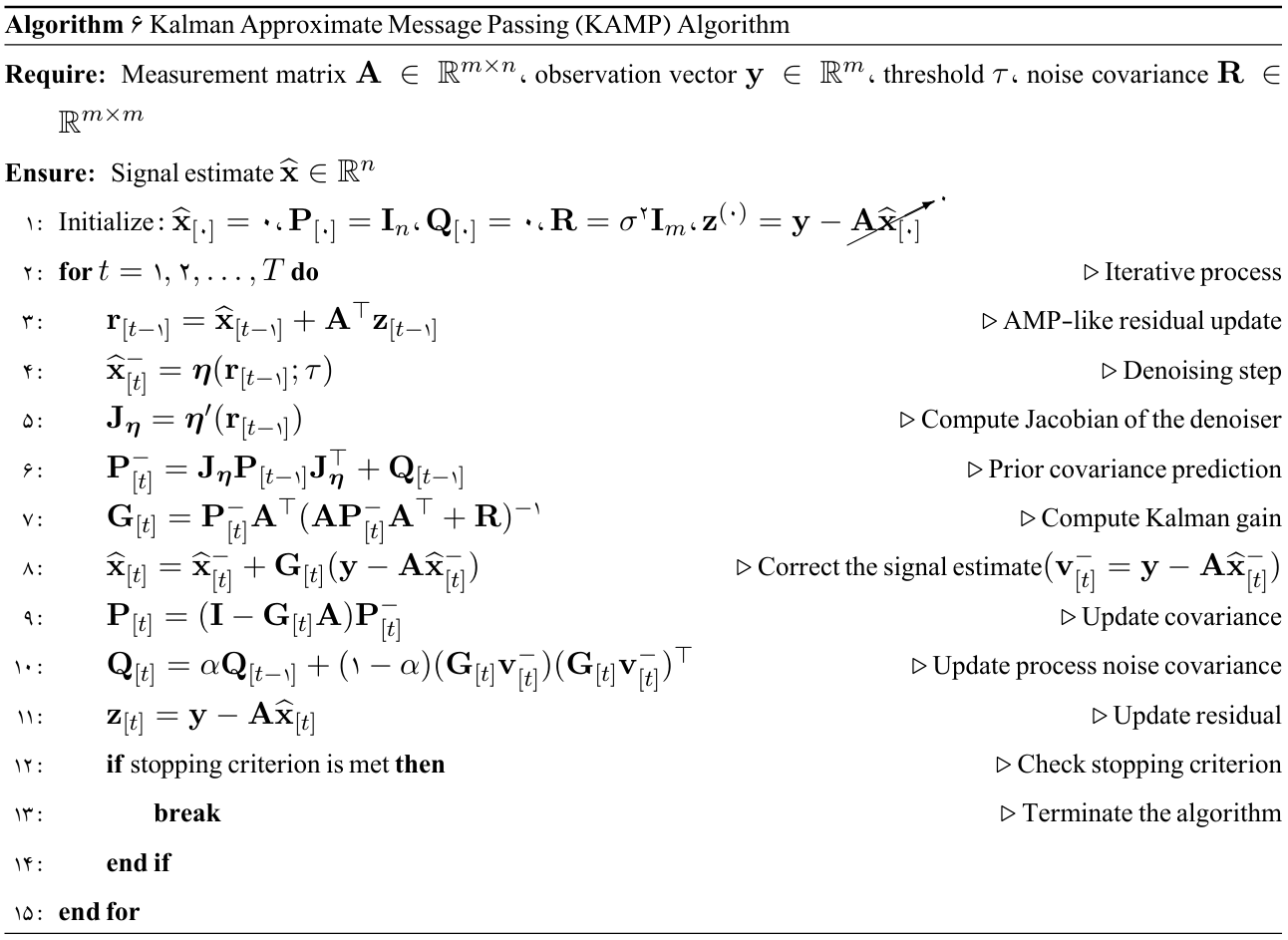
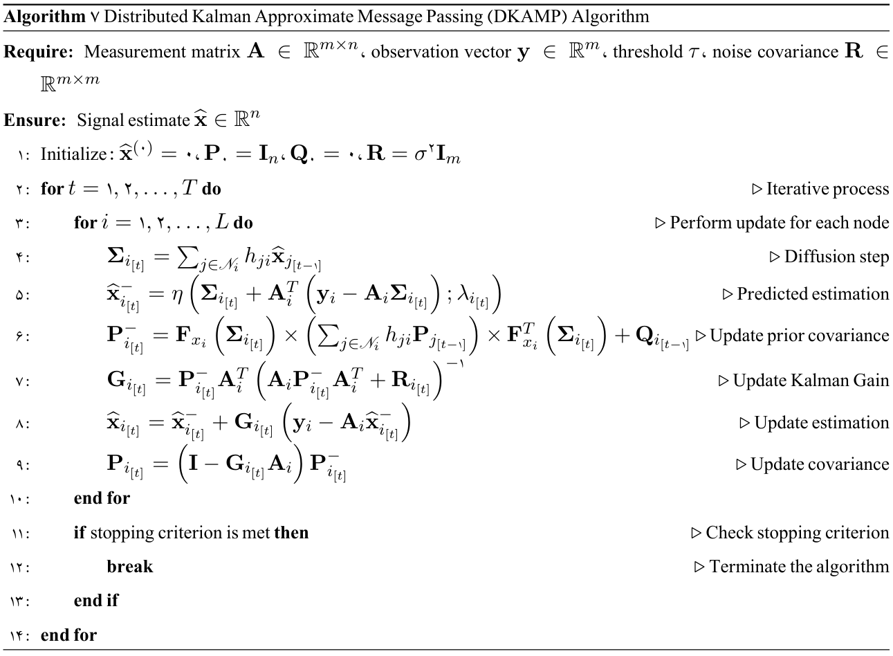
Kalman-based Approximate Message Passing Algorithm
Decentralized Version of the Proposed Method
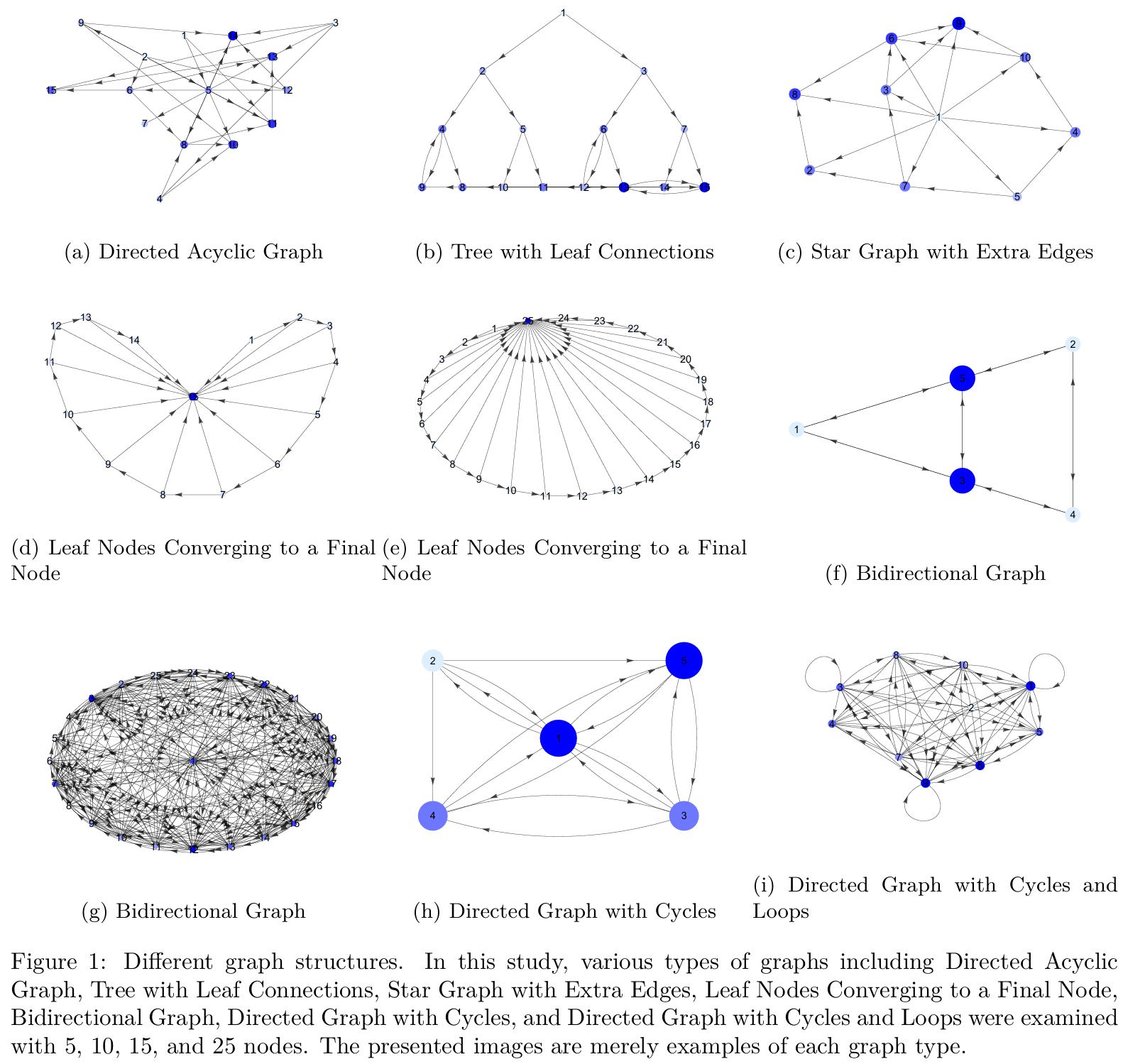
To implement algorithms such as AMP and its extended version KAMP in a decentralized manner, a network of nodes can be modeled as a directed graph $(\mathcal{G}=(\mathcal{V},\mathcal{E}))$ where $|\mathcal{V}| = L$ is the number of nodes. Each node $l$ holds a set of local observations including a submatrix $(\mathbf{A}_l)$ and a subvector $(\mathbf{y}_l)$, such that by aggregating these submatrices and vectors, the global measurement matrix and observation vector are obtained:
\[\mathbf{A} = \begin{bmatrix} \mathbf{A}_1 \\ \mathbf{A}_2 \\ \vdots \\ \mathbf{A}_L \end{bmatrix}, \qquad \mathbf{y} = \begin{bmatrix} \mathbf{y}_1 \\ \mathbf{y}_2 \\ \vdots \\ \mathbf{y}_L \end{bmatrix},\]where \((\mathbf{y}_\ell = \mathbf{A}_\ell \mathbf{x} + \boldsymbol{\omega}_\ell)\)
is the local observation model of node \((\ell)\)
(the noise vector
\((\boldsymbol{\omega}_\ell)\) also has variance
\[(\sigma^2)\]). Therefore, each node observes only part of the equation \((\mathbf{y}=\mathbf{A}\mathbf{x} + \boldsymbol{\omega})\)
and does not need to know the entire matrix
\[(\mathbf{A})\]or vector
\((\mathbf{y})\) .
In the distributed KAMP algorithm, each node runs KAMP on its local data and obtains an initial estimate of vector $(\mathbf{x})$. Then, in order to reach a joint estimate, nodes exchange their results with neighbors. A common mechanism for this exchange is consensus averaging of neighbors’ values; in this way, each node $l$ combines its own estimate with the estimates received from its neighbors $(\mathscr{N}_l)$.
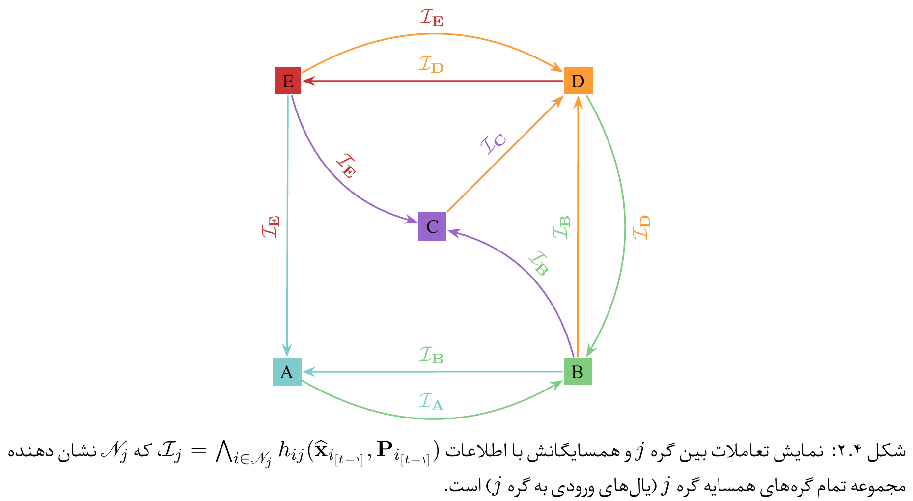
Displaying the interactions between node $j$ and its neighbors with information
\[\mathcal{I}_{j} = \bigwedge_{i \in \mathscr{N}_j} h_{ij}(\hat{\mathbf{x}}_{i_{[t-1]}}, \mathbf{P}_{i_{[t-1]}})\], where
$\mathscr{N}_j$ denotes the set of all neighbor nodes of node $j$ (incoming edges to node $j$).
Decentralized Version of the Proposed Algorithm
Decentralized Kalman-based Approximate Message Passing Algorithm
Experiments
Evaluating the Performance of the Proposed Method on the ODDS Dataset
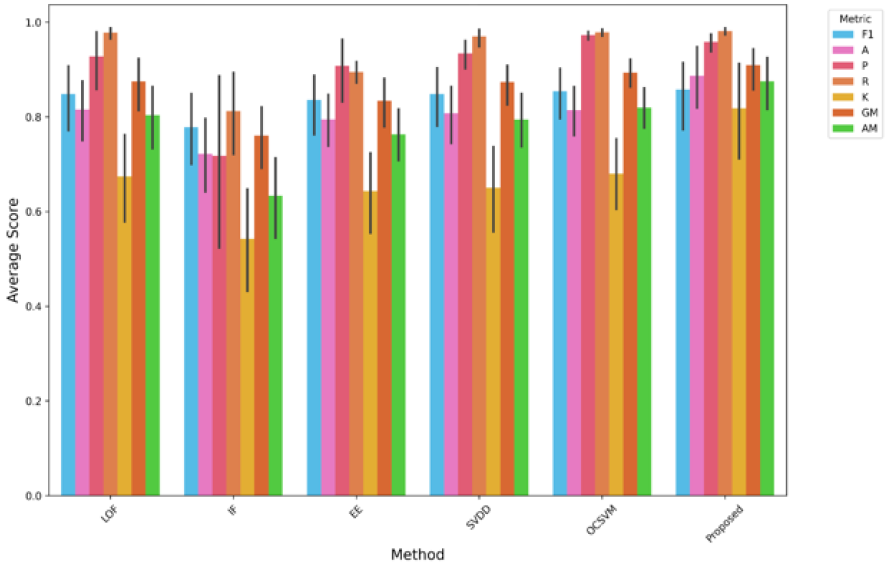
Comparison of performance metrics for different anomaly detection models, including LOF, IF, EE, SVDD, OCSVM, and the proposed method. Metrics such as F1-score (F1), Precision (P), Accuracy (A), Recall (R), Kappa (K), Geometric Mean (GM), and Arithmetic Mean (AM) are used to evaluate the effectiveness of each model. The bar chart shows the average performance scores along with error bars. The proposed method consistently achieves high scores across multiple metrics, demonstrating its strong performance and reliability compared to other models.
Evaluating the Boundary Performance of the Proposed Method on Image Data
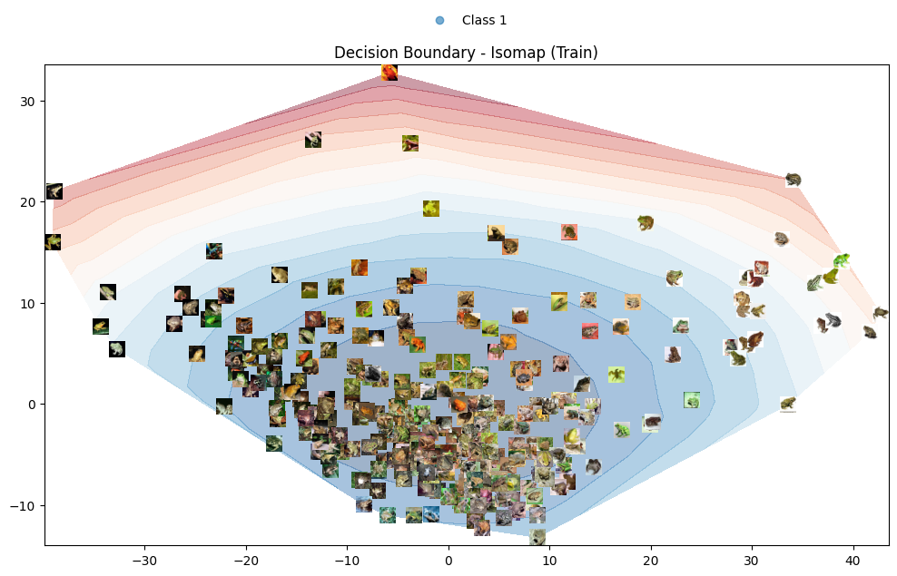
Figure 1: Decision boundary on the target class of the CIFAR-10 dataset using Isomap mapping.
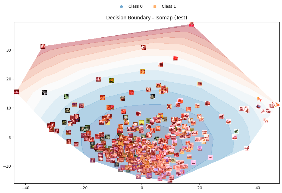
Figure 2: Decision boundary on CIFAR-10 data using Isomap mapping (all CIFAR-10 dataset classes are used).
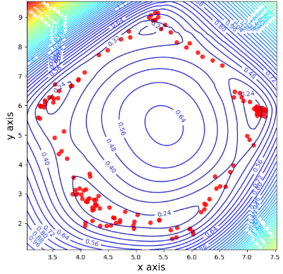
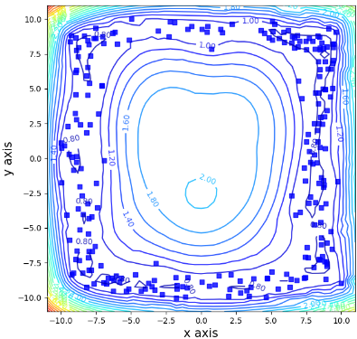
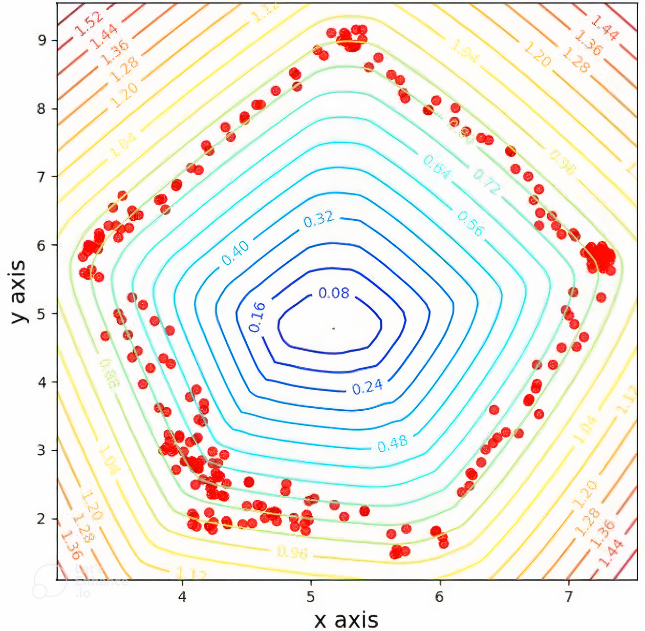
Evaluating the Flexibility of the Proposed Method in the Input Space
Proof of the Superiority of the Kalman-based Method over Approximate Message Passing
The simulations have been performed on Gaussian, orthogonal, and heavy-tailed random matrices.
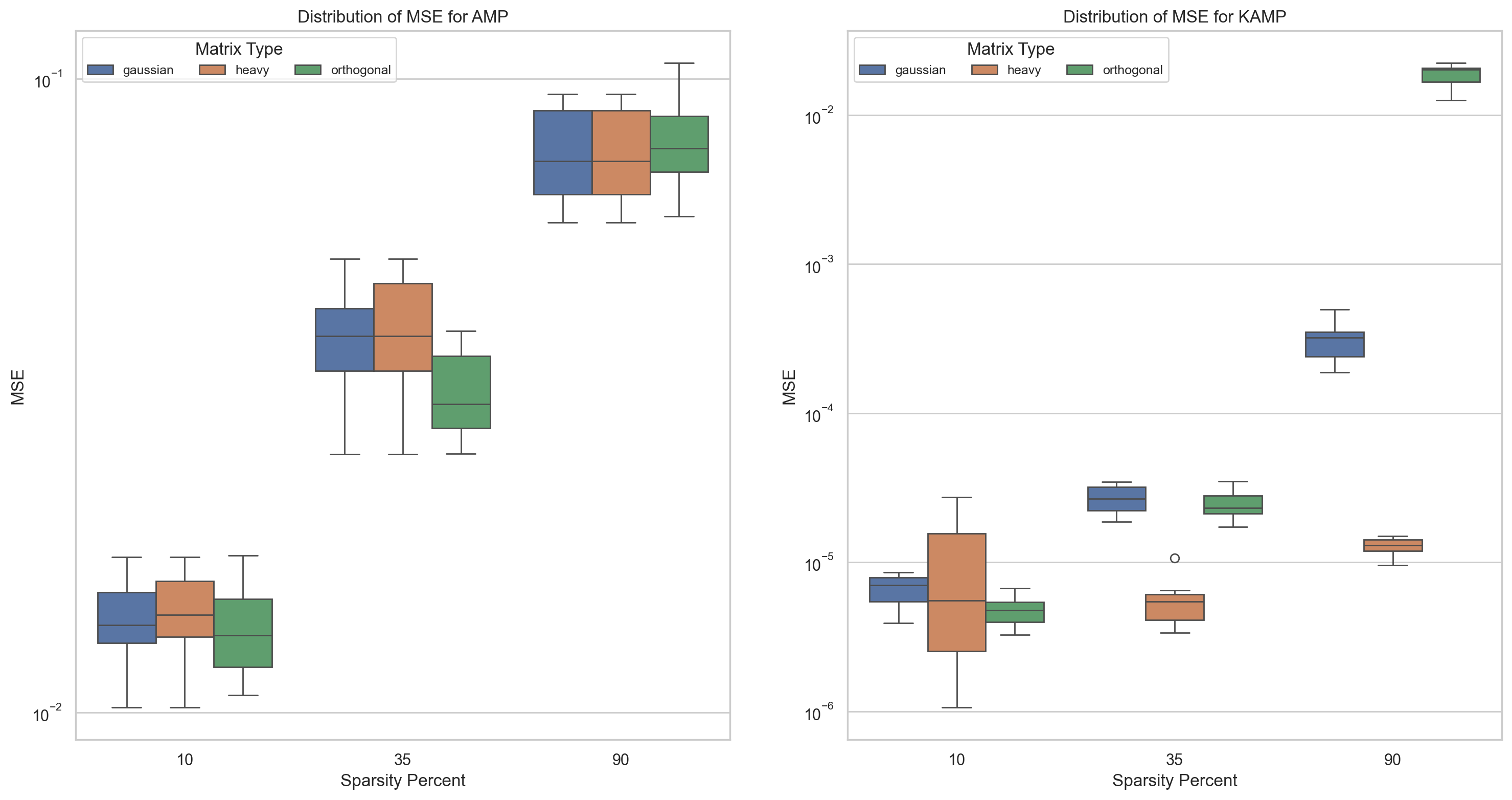
Kalman-based version achieving tighter error bounds
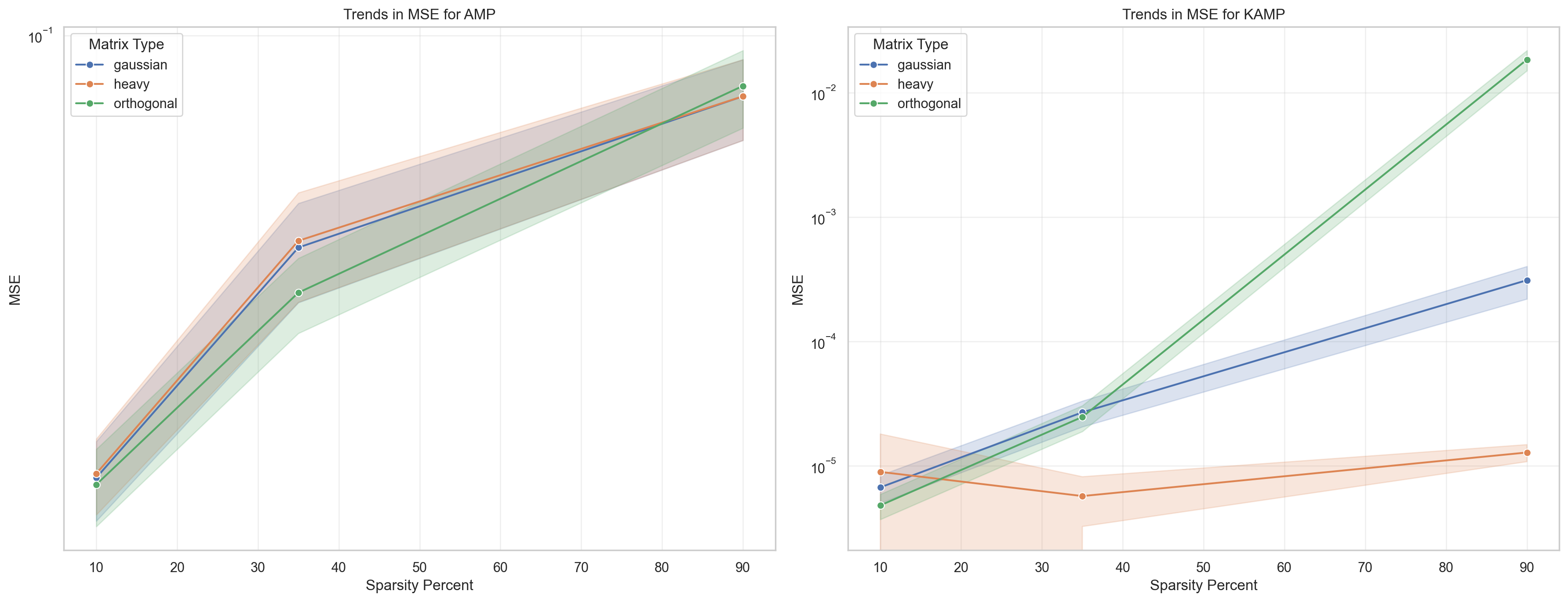
Kalman-based version achieving lower error variance
Table 1: Comparison of mean ranks and test statistics by matrix type based on the Mean Squared Error criterion
| Matrix Type | Ranks: method | Ranks: N | Ranks: Mean Rank | Test Statistics: Mann-Whitney U | Test Statistics: Wilcoxon W | Test Statistics: Z | Test Statistics: Asymp. Sig. (2-tailed) |
|---|---|---|---|---|---|---|---|
| Gaussian | AMP | 30 | 45.50 | 0.000 | 465.000 | -6.653 | < 0.001 |
| KAMP | 30 | 15.50 | |||||
| Heavy | AMP | 29 | 44.72 | 8.000 | 473.000 | -6.474 | < 0.001 |
| KAMP | 30 | 15.77 | |||||
| Orthogonal | AMP | 30 | 42.73 | 83.000 | 548.000 | -5.426 | < 0.001 |
| KAMP | 30 | 18.27 |
Table 2: Comparison of mean ranks and test statistics by matrix type based on the Signal-to-Noise Ratio criterion
| Matrix Type | Ranks: method | Ranks: N | Ranks: Mean Rank | Test Statistics: Mann-Whitney U | Test Statistics: Wilcoxon W | Test Statistics: Z | Test Statistics: Asymp. Sig. (2-tailed) |
|---|---|---|---|---|---|---|---|
| Gaussian | AMP | 30 | 15.50 | 0.000 | 465.000 | -6.653 | < 0.001 |
| KAMP | 30 | 45.50 | |||||
| Heavy | AMP | 29 | 15.00 | 0.000 | 435.000 | -6.595 | < 0.001 |
| KAMP | 30 | 44.50 | |||||
| Orthogonal | AMP | 30 | 15.50 | 0.000 | 465.000 | -6.653 | < 0.001 |
| KAMP | 30 | 45.50 |
Table 3: Comparison of mean ranks and test statistics by matrix type based on the Peak Signal-to-Noise Ratio criterion
| Matrix Type | Ranks: method | Ranks: N | Ranks: Mean Rank | Test Statistics: Mann-Whitney U | Test Statistics: Wilcoxon W | Test Statistics: Z | Test Statistics: Asymp. Sig. (2-tailed) |
|---|---|---|---|---|---|---|---|
| Gaussian | AMP | 30 | 15.50 | 0.000 | 465.000 | -6.653 | < 0.001 |
| KAMP | 30 | 45.50 | |||||
| Heavy | AMP | 29 | 15.31 | 9.000 | 444.000 | -6.459 | < 0.001 |
| KAMP | 30 | 44.20 | |||||
| Orthogonal | AMP | 30 | 18.33 | 85.000 | 550.000 | -5.396 | < 0.001 |
| KAMP | 30 | 42.67 |
Based on the conducted statistical tests, it can be seen that the proposed method consistently maintains its superiority over the AMP method in all cases.
An Example of the Examined Topologies

Ranking of the performance of different network topologies based on global network metrics
Results
- Superiority of the proposed method in one-class anomaly detection compared to competing methods
- Ability to form fully flexible boundaries in the input space
- Ability to construct a convex hull in high-dimensional feature space using a polynomial kernel
- Demonstrated efficiency of the KAMP method on different types of random matrices compared to AMP
- Achieving significantly lower error variance than the error variance of AMP
More details in the Master’s thesis of Yousof Ghalenoei from Ferdowsi University of Mashhad